Quantum Fundamentals: Winter-2026
HW3 (SOLUTION): Due W2 D3
- Eigenvectors of the Rotation Matrix
S1 5473S
The orthogonal matrix
\[R_z(\theta)=
\begin{pmatrix}
\cos\theta&-\sin\theta&0\\ \sin\theta&\cos\theta&0\\ 0&0&1\\
\end{pmatrix}
\]
corresponds to a rotation around the \(z\)-axis by the angle \(\theta\).
- Find the eigenvalues of this matrix.
\begin{eqnarray*} 0 &=& \left\vert \begin{pmatrix} \lambda-\cos\theta&\sin\theta&0\\ -\sin\theta&\lambda-\cos\theta&0\\0&0&\lambda-1\\ \end{pmatrix} \right\vert \\ {} &=& (\lambda-\cos\theta)^2(\lambda-1)+(\lambda-1)\sin^2\theta \\ {} &=& (\lambda-1)(\lambda^2-2\lambda\cos\theta+1) \\ {} &\Rightarrow& \lambda=1, \lambda=\cos\theta\pm i\sin\theta = e^{\pm i\theta} \end{eqnarray*}
- Find the normalized eigenvectors of this matrix.
The eigenvector corresponding to \(\lambda=1\) is given by: \[ \begin{pmatrix} \cos\theta&-\sin\theta&0\\\sin\theta&\cos\theta&0\\0&0&0\\ \end{pmatrix} \begin{pmatrix} x\\ y\\ z\\ \end{pmatrix} = \begin{pmatrix} x\\ y\\ z\\ \end{pmatrix} \Rightarrow v_1= \begin{pmatrix} 0\\ 0\\ 1\\ \end{pmatrix} \] (The two equations for \(x\) and \(y\) require \(x=y=0\).) The vector is already normalized. The eigenvectors corresponding to \(\lambda=e^{\pm i\theta}\) are given by: \[ \begin{pmatrix} \cos\theta&-\sin\theta&0\\\sin\theta&\cos\theta&0\\0&0&1\\ \end{pmatrix} \begin{pmatrix} x\\ y\\ z\\ \end{pmatrix} = e^{\pm i\theta} \begin{pmatrix} x\\ y\\ z\\ \end{pmatrix} \Rightarrow v_{\pm} =\frac{1}{\sqrt{2}} \begin{pmatrix} 1\\ \mp i\\ 0\\ \end{pmatrix} \] The factor \(1/\sqrt{2}\) is inserted so that the vector is normalized, i.e. \(|x|^2+|y|^2+|z|^2=1\).
- Describe how the eigenvectors do or do not correspond to the vectors
which are held constant or “only stretched” by this
transformation.
The eigenvector corresponding to the eigenvalue \(1\) is just \( \begin{pmatrix} 0\\0\\1 \end{pmatrix} \). It points along the \(z\)-axis, the axis of rotation. This is the only real direction which is fixed by the rotation, that is what you mean by an axis of rotation. The other two eigenvectors correspond to complex eigenvalues \(\lambda=e^{\pm i\theta}\). The eigenvectors themselves \(v_{\pm} = \begin{pmatrix} 1\\ \pm i\\ 0\\ \end{pmatrix}\) are not real, and hence do not correspond to real directions in real 3-dimensional space. These vectors are only “stretched” during the transformation in that they scale by the complex factor \(e^{\pm i\theta}\).
- Find the eigenvalues of this matrix.
- Stern Gerlach Explain
S1 5473S
Use words and equations to explain the key features of the Stern-Gerlach experiment.
The Stern-Gerlach experiment involves firing electrically neutral particles with a non-zero magnetic momentum through an inhomogeneous magnetic field. This inhomogeneity means that (at least) one of magnetic field's components has a nonzero gradient. The particles will then feel a force according to \begin{eqnarray*} \vec{F} &=& -\vec{\nabla} (-\vec{\mu} \cdot \vec{B})\\ &=& \mu_x \vec{\nabla} B_x(x,y,z) + \mu_y \vec{\nabla} B_y(x,y,z) + \mu_z \vec{\nabla} B_z(x,y,z) \end{eqnarray*}
An inhomogenous magnetic field will cause the particles for feel a force. Since magnetic moment is related to momentum: \[\vec{\mu} = \frac{gp}{2m} \vec{S}\] particles with different angular momentum will be accelerated differently, causing them to hit a screen in different locations.
Contrast Classical/Quantum Explain what you would predict based only on classical physics for the Stern-Gerlach experiment and describe the difference between the classical prediction and the actual experimental results.
Classically we would expect a continuum of spin angular momentum \(\vec{S}\) coming out of the oven. The force acting on the particles is \begin{eqnarray*} F_z \approx g \frac{-e}{2m_e} S_z \frac{\partial B_z}{\partial z} \end{eqnarray*}
Since the force depends on \(z\) component of the angular momentum, we would expect to see a broad smearing of where the atoms strike the targets.
We see something very different experimentally - the locations where the atoms strike the target are not continuous at all! We see instead two distinct bands where the atoms strike the target, informing us that the atoms (or, more specifically, the single electron in the valance shell of the silver atoms) have only two possible values for the spin angular momentum. We would say that the spin angular momentum is quantized.
- Statistical Analysis of the Spins Sim
S1 5473S
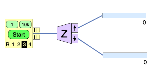
In the spins sim, the oven can be set to emit particles in a particular unknown prepared state (instead of in a random state).
- Set the oven to Unknown #3.
- Orient the analyzer in the \(z\)-direction.
- Perform 5 sets of 10,000 Stern-Gerlach experiments (10,000 particles are sent through a Stern-Gerlach Analyzer) and record the number of particles that end up in the top counter.
- For each set of experiments, calculate the probability that a single particle was measured to have \(S_z = +\hbar/2\).
Do all of the following calculations by hand (you can use a calculator to help with the arithmetic).
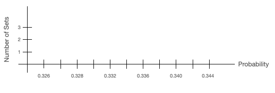
Plot a histogram of the probabilities you measured for each set. Use a bin size of 0.002 for the horizontal axis. (Choose appropriate values on the horizontal axis. You don't need to plot the full possible values 0-1. You may use a computer to make the histogram or you can sketch it by hand.)
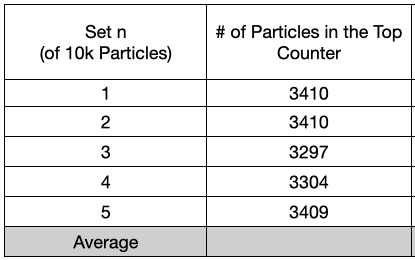
My data is:
My histogram looks like:
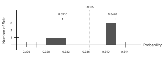
What is your best estimate of the probability that, when you measure \(S_z\) of a particle in the Unknown #3 state, you will get a result of \(+\hbar/2\)? Mark this value on your histogram.
The best estimate of the probability is the average of the probabilities:
\begin{align*} \bar{\mathcal{P}} &= \frac{1}{5}\sum_{n=1}^5 P_n \\ &= \frac{(0.3410+0.3410+0.3297+0.3304+0.3409)}{5} \\ &= 0.3365 \end{align*}