Quantum Fundamentals: Winter-2026
HW 6 (SOLUTION): Due W3 D5
- Measurement Probabilities (Brief)
S1 5420S
A beam of spin-\(\frac{1}{2}\) particles is prepared in the initial state \[ \left\vert \psi\right\rangle = \sqrt{\frac{2}{5}}\; |+\rangle_x - \sqrt{\frac{3}{5}}\; |-\rangle_x \](Note: this state is written in the \(S_x\) basis!)
- What are the possible measurement values if you measure the spin component \(S_x\), and with what probabilities would they occur?
The possible measurement values are \(S_x=+\hbar/2\) and \(S_x=-\hbar/2\) The probabilities of getting these values are found by taking the norm squared of the expansion coefficients: The probability of measuring \(\hbar/2\) is: \begin{align*} \mathcal{P}\left(S_x=+\frac{\hbar}{2}\right) =& \left|{}_x\left\langle {+}\middle|{\psi}\right\rangle \right|^2 \\ =& \left|\sqrt{\frac{2}{5}}\right|^2 \\ =& \frac{2}{5} \end{align*}
The probability of measuring \(-\hbar/2\) is: \begin{align*} \mathcal{P}\left(S_x=-\frac{\hbar}{2}\right) =& \left|{}_x\left\langle {-}\middle|{\psi}\right\rangle \right|^2 \\ =&\left|-\sqrt{\frac{3}{5}} \right|^2 \\ =& \frac{3}{5} \end{align*} (Check: \(2/5 + 3/5 = 1\)).
- What are the possible measurement values if you measure the spin component \(S_z\), and with what probabilities would they occur?
The possible measurement values are \(S_z=+\hbar/2\) and \(S_z=-\hbar/2\) The probabilities of getting these values are found by taking the norm squared of the inner product between the state and z-basis states: The probability of measuring \(\hbar/2\) is \begin{align*} \mathcal{P}\left(S_z=\frac{\hbar}{2}\right) =& \left|\left\langle {+}\middle|{\psi}\right\rangle \right|^2\\ =&\left|\langle+| \left( \sqrt{\frac{2}{5}} |+\rangle_x - \sqrt{\frac{3}{5}} |-\rangle_x \right)\right|^2\\ =& \left|\left( \sqrt{\frac{2}{5}} \langle+|+\rangle_x - \sqrt{\frac{3}{5}} \langle+|-\rangle_x \right)\right|^2\\ =& \left|\left(\sqrt{\frac{2}{5}} \left(\frac{1}{\sqrt{2}}\right) - \sqrt{\frac{3}{5}} \left(\frac{1}{\sqrt{2}}\right)\right)\right|^2\\ =& \left|\sqrt{\frac{2}{10}} - \sqrt{\frac{3}{10}}\right|^2\\ =& \frac{5-2\sqrt{6}}{10}\\ \approx& 0.01 \end{align*}
The probability of measuring \(-\hbar/2\) is \begin{align*} \mathcal{P}\left(S_z=-\frac{\hbar}{2}\right) =& \left|\left\langle {-}\middle|{\psi}\right\rangle \right|^2\\ \left|\langle-|\left(\sqrt{\frac{2}{5}} |+\rangle_x - \sqrt{\frac{3}{5}} |-\rangle_x\right)\right|^2 =& \left|\left(\sqrt{\frac{2}{5}} \langle-|+\rangle_x - \sqrt{\frac{3}{5}} \langle-|-\rangle_x\right)\right|^2\\ =& \left|\left(\sqrt{\frac{2}{5}} \left(\frac{1}{\sqrt{2}}\right) - \sqrt{\frac{3}{5}} \left(-\frac{1}{\sqrt{2}}\right)\right)\right|^2\\ =& \left|\sqrt{\frac{2}{10}} + \sqrt{\frac{3}{10}}\right|^2\\ =& \frac{5+2\sqrt{6}}{10}\\ \approx& 0.99 \end{align*}
(Check: \(0.01 + 0.99 = 1\)).
- What are the possible measurement values if you measure the spin component \(S_x\), and with what probabilities would they occur?
- Completeness Relation Change of Basis
S1 5420S
Given the polar basis kets written as a superposition of Cartesian kets \begin{eqnarray*} \left|{\hat{s}}\right\rangle &=& \cos\phi \left|{\hat{x}}\right\rangle + \sin\phi \left|{\hat{y}}\right\rangle \\ \left|{\hat{\phi}}\right\rangle &=& -\sin\phi \left|{\hat{x}}\right\rangle + \cos\phi \left|{\hat{y}}\right\rangle \end{eqnarray*}
Find the following quantities: \[\left\langle {\hat{x}}\middle|{\hat{s}}\right\rangle ,\quad \left\langle {\hat{y}}\middle|{{\hat{s}}}\right\rangle ,\quad \left\langle {\hat{x}}\middle|{\hat{\phi}}\right\rangle ,\quad \left\langle {\hat{y}}\middle|{\hat{\phi}}\right\rangle \]
To find \(\left\langle {\hat{x}}\middle|{\hat{s}}\right\rangle \) we need to perform the inner product. \[\left\langle {\hat{x}}\middle|{\hat{s}}\right\rangle = \left\langle {\hat{x}}\right|(\cos\phi \left|{\hat{x}}\right\rangle + \sin\phi \left|{\hat{y}}\right\rangle )\] \[\left\langle {\hat{x}}\middle|{\hat{s}}\right\rangle = \cos\phi \left\langle {\hat{x}}\middle|{\hat{x}}\right\rangle + \sin\phi \left\langle {\hat{x}}\middle|{\hat{y}}\right\rangle \] Because the Cartesian basis vectors are orthonormal \(\left\langle {\hat{x}}\middle|{\hat{x}}\right\rangle = 1\) and \(\left\langle {\hat{x}}\middle|{\hat{y}}\right\rangle = 0\) which lets our answer simplify to \[\left\langle {\hat{x}}\middle|{\hat{s}}\right\rangle = \cos\phi\] We see that this is just the coefficient of the \(\left|{\hat{x}}\right\rangle \) bit of \(\left|{\hat{s}}\right\rangle \). Similarly the rest of the desired quanties are as follows: \begin{eqnarray*} \left\langle {\hat{y}}\middle|{\hat{s}}\right\rangle &= \sin\phi \\ \left\langle {\hat{x}}\middle|{\hat{\phi}}\right\rangle &= -\sin\phi \\ \left\langle {\hat{y}}\middle|{\hat{\phi}}\right\rangle &= \cos\phi \end{eqnarray*}
- Given a vector written in the polar basis
\[\left|{\vec{v}}\right\rangle = a\left|{\hat{s}}\right\rangle + b\left|{\hat{\phi}}\right\rangle \]
where \(a\) and \(b\) are known.
Express \(\left|{\vec{v}}\right\rangle \) in the Cartesian basis, \[\left|{\vec{v}}\right\rangle = c\left|{\hat{x}}\right\rangle + d\left|{\hat{y}}\right\rangle \] by finding \(c\) and \(d\)
Hint: Use the completeness relation: \(\left|{\hat{x}}\right\rangle \left\langle {\hat{x}}\right| + \left|{\hat{y}}\right\rangle \left\langle {\hat{y}}\right| = 1\)Let's multiply both sides of \(\left|{\vec{v}}\right\rangle \) by \(1\) in the form of the completeness relation \[(\left|{\hat{x}}\right\rangle \left\langle {\hat{x}}\right| + \left|{\hat{y}}\right\rangle \left\langle {\hat{y}}\right|)(\left|{\vec{v}}\right\rangle ) = (\left|{\hat{x}}\right\rangle \left\langle {\hat{x}}\right| + \left|{\hat{y}}\right\rangle \left\langle {\hat{y}}\right|)(a\left|{\hat{s}}\right\rangle + b\left|{\hat{\phi}}\right\rangle )\] We can then distribute, being careful to keep the ordering preserved \[\left|{\hat{x}}\right\rangle \left\langle {\hat{x}}\middle|{\vec{v}}\right\rangle + \left|{\hat{y}}\right\rangle \left\langle {\hat{y}}\middle|{\vec{v}}\right\rangle = \left|{\hat{x}}\right\rangle \left\langle {\hat{x}}\right|a\left|{\hat{s}}\right\rangle + \left|{\hat{y}}\right\rangle \left\langle {\hat{y}}\right|a\left|{\hat{s}}\right\rangle + \left|{\hat{x}}\right\rangle \left\langle {\hat{x}}\right|b\left|{\hat{\phi}}\right\rangle + \left|{\hat{y}}\right\rangle \left\langle {\hat{y}}\right|b\left|{\hat{\phi}}\right\rangle \] Now we can move numbers out of our inner products \[\left|{\hat{x}}\right\rangle \left\langle {\hat{x}}\middle|{\vec{v}}\right\rangle + \left|{\hat{y}}\right\rangle \left\langle {\hat{y}}\middle|{\vec{v}}\right\rangle = \left|{\hat{x}}\right\rangle a\left\langle {\hat{x}}\middle|{\hat{s}}\right\rangle + \left|{\hat{y}}\right\rangle a \left\langle {\hat{y}}\middle|{\hat{s}}\right\rangle + \left|{\hat{x}}\right\rangle b\left\langle {\hat{x}}\middle|{\hat{\phi}}\right\rangle + \left|{\hat{y}}\right\rangle b\left\langle {\hat{y}}\middle|{\hat{\phi}}\right\rangle \] And we see that we have the change of basis inner products from the previous part \[\left|{\hat{x}}\right\rangle \left\langle {\hat{x}}\middle|{\vec{v}}\right\rangle + \left|{\hat{y}}\right\rangle \left\langle {\hat{y}}\middle|{\vec{v}}\right\rangle = \left|{\hat{x}}\right\rangle a\cos\phi + \left|{\hat{y}}\right\rangle a\sin\phi+ \left|{\hat{x}}\right\rangle b(-\sin\phi) + \left|{\hat{y}}\right\rangle b\cos\phi\] Lets group common terms \[\left|{\hat{x}}\right\rangle \left\langle {\hat{x}}\middle|{\vec{v}}\right\rangle + \left|{\hat{y}}\right\rangle \left\langle {\hat{y}}\middle|{\vec{v}}\right\rangle = \left|{\hat{x}}\right\rangle (a\cos\phi-b\sin\phi) + \left|{\hat{y}}\right\rangle (a\sin\phi+b\cos\phi)\]
Given a quantum state written in the \(S_z\) basis, \[ \left|{\Psi}\right\rangle = g \left|{+}\right\rangle + h \left|{-}\right\rangle , \] express \(\left|{\Psi}\right\rangle \) in the \(S_y\) basis. That is, find coefficients \(j\) and \(k\) such that \[ \left|{\Psi}\right\rangle = j \left|{+}\right\rangle _y + k \left|{-}\right\rangle _y. \]
[Method 1: Completeness relation] Because we want to express \(\left|{\Psi}\right\rangle \) in the \(S_y\) basis, we use the completeness relation written in that basis: \[ \left|{+}\right\rangle _y{_y}\left\langle {+}\right| + \left|{-}\right\rangle _y{_y}\left\langle {-}\right| = 1. \]
Multiplying this form of \(1\) onto the state \(\left|{\Psi}\right\rangle \) gives \[ \left|{\Psi}\right\rangle = \left(\left|{+}\right\rangle _y{_y}\left\langle {+}\right| + \left|{-}\right\rangle _y{_y}\left\langle {-}\right|\right)\left|{\Psi}\right\rangle . \]
Substituting \(\left|{\Psi}\right\rangle =g\left|{+}\right\rangle +h\left|{-}\right\rangle \) on the right-hand side of the equation and distributing the products, we obtain four terms: \[ \left|{\Psi}\right\rangle = g\left|{+}\right\rangle _y{_y}\left\langle {+}\middle|{+}\right\rangle + h\left|{+}\right\rangle _y{_y}\left\langle {+}\middle|{-}\right\rangle + g\left|{-}\right\rangle _y{_y}\left\langle {-}\middle|{+}\right\rangle + h\left|{-}\right\rangle _y{_y}\left\langle {-}\middle|{-}\right\rangle . \]
Using the known inner products between the \(S_y\) basis bras and the \(S_z\) basis kets, \[ {_y}\left\langle {+}\middle|{+}\right\rangle =\frac{1}{\sqrt{2}}, \qquad {_y}\left\langle {+}\middle|{-}\right\rangle =\frac{-i}{\sqrt{2}}, \] \[ {_y}\left\langle {-}\middle|{+}\right\rangle =\frac{1}{\sqrt{2}}, \qquad {_y}\left\langle {-}\middle|{-}\right\rangle =\frac{i}{\sqrt{2}}, \] we obtain \[ \left|{\Psi}\right\rangle = \left|{+}\right\rangle _y\left(\frac{g}{\sqrt{2}}-\frac{ih}{\sqrt{2}}\right) + \left|{-}\right\rangle _y\left(\frac{g}{\sqrt{2}}+\frac{ih}{\sqrt{2}}\right). \]
Therefore, the state written in the \(S_y\) basis is \[ \left|{\Psi}\right\rangle = \frac{g-ih}{\sqrt{2}}\left|{+}\right\rangle _y + \frac{g+ih}{\sqrt{2}}\left|{-}\right\rangle _y, \] and the coefficients are \begin{eqnarray*} j = \frac{g-ih}{\sqrt{2}},\\\\ k= \frac{g+ih}{\sqrt{2}}. \end{eqnarray*}
[Method 2: Projection onto the \(S_y\) basis] Since we want to express \(\left|{\Psi}\right\rangle \) in the \(S_y\) basis, the coefficients are given by the scalar projections of \(\left|{\Psi}\right\rangle \) onto the \(S_y\) basis states.
That is, \begin{eqnarray*} j &=& {_y}\left\langle {+}\middle|{\Psi}\right\rangle , \\ k &=& {_y}\left\langle {-}\middle|{\Psi}\right\rangle . \end{eqnarray*}
Using \(\left|{\Psi}\right\rangle =g\left|{+}\right\rangle +h\left|{-}\right\rangle \), we first write the scalar projections explicitly: \[ {_y}\left\langle {+}\middle|{\Psi}\right\rangle = {_y}\left\langle {+}\right|\left(g\left|{+}\right\rangle +h\left|{-}\right\rangle \right), \qquad {_y}\left\langle {-}\middle|{\Psi}\right\rangle = {_y}\left\langle {-}\right|\left(g\left|{+}\right\rangle +h\left|{-}\right\rangle \right). \]
Pulling the scalar coefficients outside the inner products gives \[ {_y}\left\langle {+}\middle|{\Psi}\right\rangle = g\,{_y}\left\langle {+}\middle|{+}\right\rangle + h\,{_y}\left\langle {+}\middle|{-}\right\rangle , \] \[ {_y}\left\langle {-}\middle|{\Psi}\right\rangle = g\,{_y}\left\langle {-}\middle|{+}\right\rangle + h\,{_y}\left\langle {-}\middle|{-}\right\rangle . \]
Using the known inner products, \[ {_y}\left\langle {+}\middle|{+}\right\rangle =\frac{1}{\sqrt{2}}, \qquad {_y}\left\langle {+}\middle|{-}\right\rangle =\frac{-i}{\sqrt{2}}, \] \[ {_y}\left\langle {-}\middle|{+}\right\rangle =\frac{1}{\sqrt{2}}, \qquad {_y}\left\langle {-}\middle|{-}\right\rangle =\frac{i}{\sqrt{2}}, \] we obtain \[ {_y}\left\langle {+}\middle|{\Psi}\right\rangle = \frac{g}{\sqrt{2}} - \frac{i h}{\sqrt{2}} = \frac{g-ih}{\sqrt{2}}, \] \[ {_y}\left\langle {-}\middle|{\Psi}\right\rangle = \frac{g}{\sqrt{2}} + \frac{i h}{\sqrt{2}} = \frac{g+ih}{\sqrt{2}}. \]
Therefore, \[ j={_y}\left\langle {+}\middle|{\Psi}\right\rangle =\frac{g-ih}{\sqrt{2}}, \qquad k={_y}\left\langle {-}\middle|{\Psi}\right\rangle =\frac{g+ih}{\sqrt{2}}. \]
- Spin One Intro
S1 5420S
The OSP Spins Laboratory simulation can also be used to explore spin-1 systems. The components of spin for these systems can be measured to be:
\(\hbar\) (corresponding to the “+” port)
\(0\hbar\) (corresponding to the “0” port)
\(-\hbar\) (corresponding to the “-” port)
To switch the simulation to a spin-1 system, find the hyperlink about halfway down the page that says “Click here to switch”.
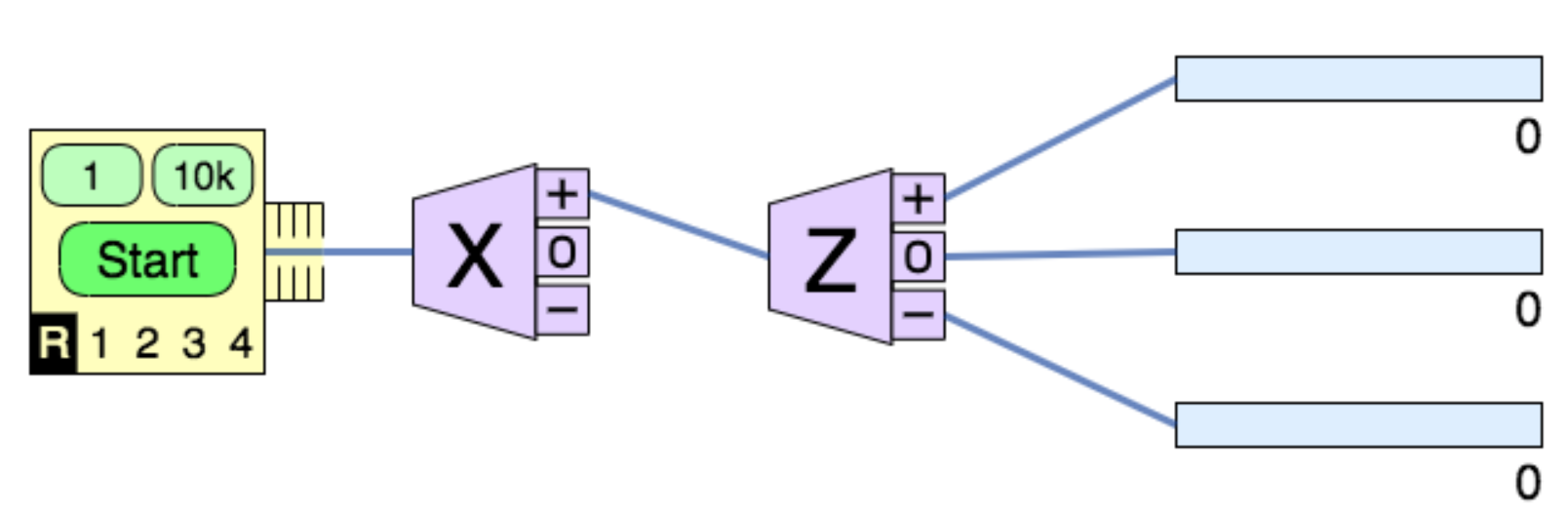
Draw and label a diagram of an experimental setup that would allow you to prepare a set of spin-1 particles to be in the \(|1\rangle_x\) state and than measure the \(z\) component of spin for these particles.
To prepare a particle in the \(\left|{1}\right\rangle _x\) state, I need to make a measurement of the \(x\)-component of spin. I will set up a SG analyzer (i.e., a polarizer) oriented in the \(x\)-direction and select the particles with \(S_x = \hbar\) to go into a second analyzer oriented in the \(z\) direction to measure the \(z\)-components of spin.
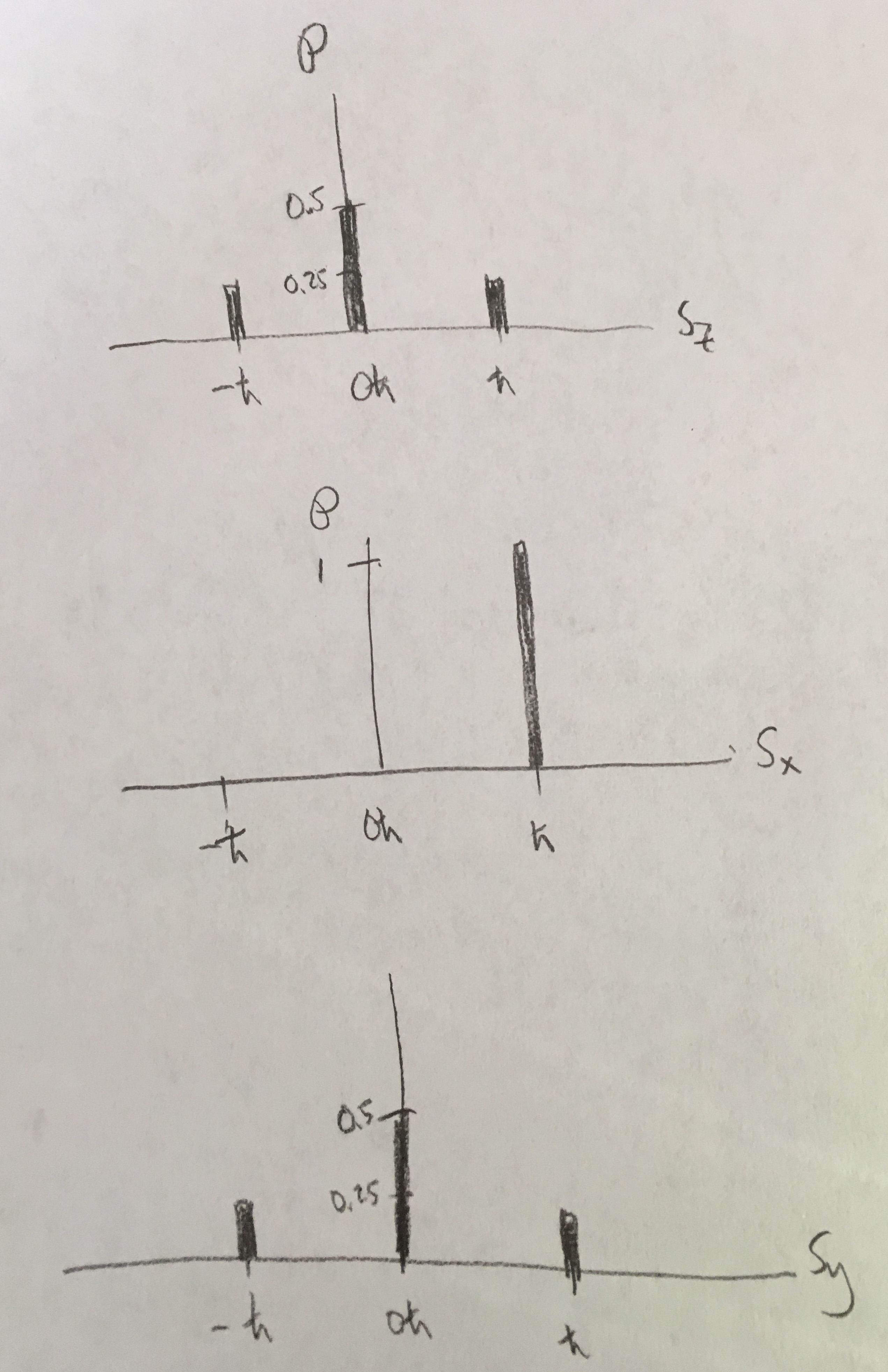
Using the simulation, prepare a set of particles to be in the \(|1\rangle_x\) state and measure the \(x\), \(y\), and \(z\) components of spin of these particles. Draw probability histograms of the results for each spin-component-direction \(S_x\), \(S_y\), and \(S_z\).
I will use the experiment shown in part a) but change the orientation of the second analyzer to be in the \(x\) and \(y\) directions as needed. The histograms will look like: