Quantum Fundamentals: Winter-2026
HW 4 (SOLUTION): Due W2 D5
- Histogram
S1 5416S
Note: The states \(\lvert + \rangle_z\) and \(\lvert - \rangle_z\) are often written without the subscript \(z\) as \(\lvert + \rangle\) and \(\lvert - \rangle\). The subscripts are not omitted for the states \(\lvert + \rangle_x\), \(\lvert - \rangle_x\), \(\lvert + \rangle_y\), and \(\lvert - \rangle_y\).
A beam of spin-\(\frac{1}{2}\) particles is prepared in the state: \[\left\vert \psi\right\rangle = \frac{2}{\sqrt{13}}\left\vert +\right\rangle+ i\frac{3}{\sqrt{13}} \left\vert -\right\rangle\]
- What are the possible measurement values if you measure the spin component \(S_z\), and with what probabilities would they occur? Check Beasts: Check that you have the right “beast.”
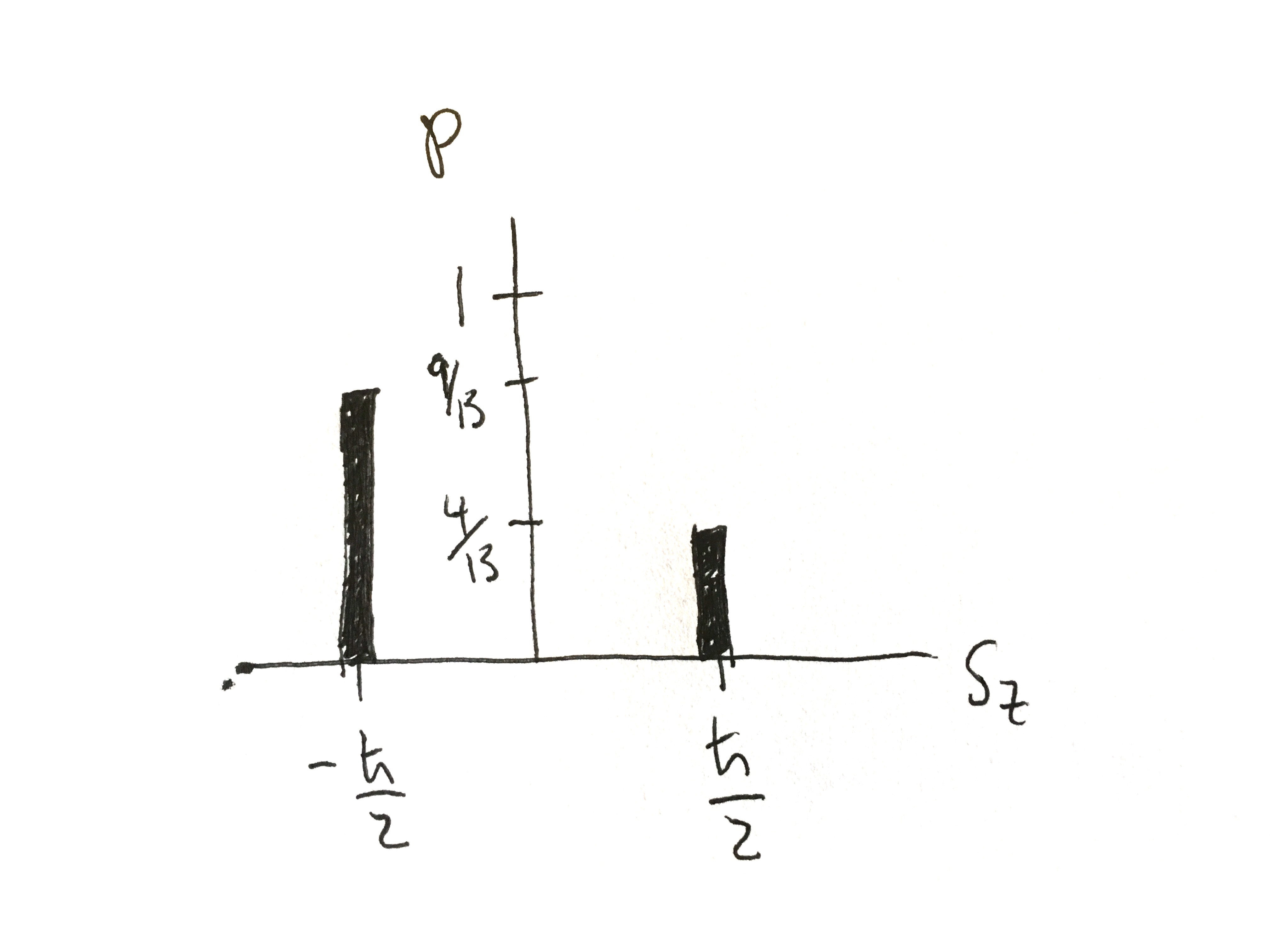
The (normalized) state we are given is \(\left|{\psi}\right\rangle = \frac{2}{\sqrt{13}} \left|{+}\right\rangle + i\frac{3}{\sqrt{13}}\left|{-}\right\rangle \), where \(\{\left|{+}\right\rangle ,\left|{-}\right\rangle \}\) is the spin-1/2 z-basis. The possible values of the measurement of the \(z\)-component of angular momentum, i.e. \(\pm(\hbar/2)\). You just have to know this. There is nothing to calculate. The probabilities to get them in a measurement are given by the squares of the norms of the coefficients in the expansion (of the particular state) in this basis. Since the state itself is already given in that basis, the probabilities are simply the squares of the norms of the coefficients, ie. \begin{align*} \mathcal{P}_+ =& \vert\left\langle {+}\middle|{\psi}\right\rangle \vert^2=\left|\frac{2}{\sqrt{13}}\right|^2\\ =& \frac{4}{13} \\ \mathcal{P}_- =& \vert\left\langle {-}\middle|{\psi}\right\rangle \vert^2 =\left|i \frac{3}{\sqrt{13}}\right|^2 \\ =& \frac{9}{13} \end{align*} These coefficients are positive, real scalars that add up to \(1\), as they ought to. (Since these are the only possible values/states, we must find one of them in a measurement.)
- What are the possible measurement values if you measure the spin component \(S_x\), and with what probabilities would they occur? Check Beasts: Check that you have the right “beast.”
The possible values that can be measured are again \(\pm \frac{\hbar}{2}\). Getting them in a measurement means ending up in the respective eigenstate, \(\left|{+}\right\rangle _x\) or \(\left|{-}\right\rangle _x\). The probability of this happening, for the given state \(\left|{\psi}\right\rangle \), can be obtained as \begin{align*} \mathcal{P}_{+x} =& \left|{}_x\left\langle {+}\middle|{\psi}\right\rangle \right|^2\\ \mathcal{P}_{-x} =& \left|{}_x\left\langle {-}\middle|{\psi}\right\rangle \right|^2\\ \end{align*}
This can also be stated as follows. If the state \(\left|{\psi}\right\rangle \) is written in terms of \(\,\widehat{\!S}_x\), which is \(\{\left|{+}\right\rangle _x, \left|{-}\right\rangle _x\}\), the probabilities are found from the expansion coefficients (by squaring their absolute values). The coefficients are precisely \({}_x\left\langle {\pm}\middle|{\psi}\right\rangle \). The \(|+\rangle_x\) coefficient is: \begin{align*} {}_x\left\langle {+}\middle|{\psi}\right\rangle =& \frac{2}{\sqrt{13}} {}_x\left\langle {+}\middle|{+}\right\rangle + i \frac{3}{\sqrt{13}} {}_x\left\langle {+}\middle|{-}\right\rangle \\ =& \frac{2}{\sqrt{2}\sqrt{13}} + \frac{3\,i}{\sqrt{2}\sqrt{13}} \end{align*}
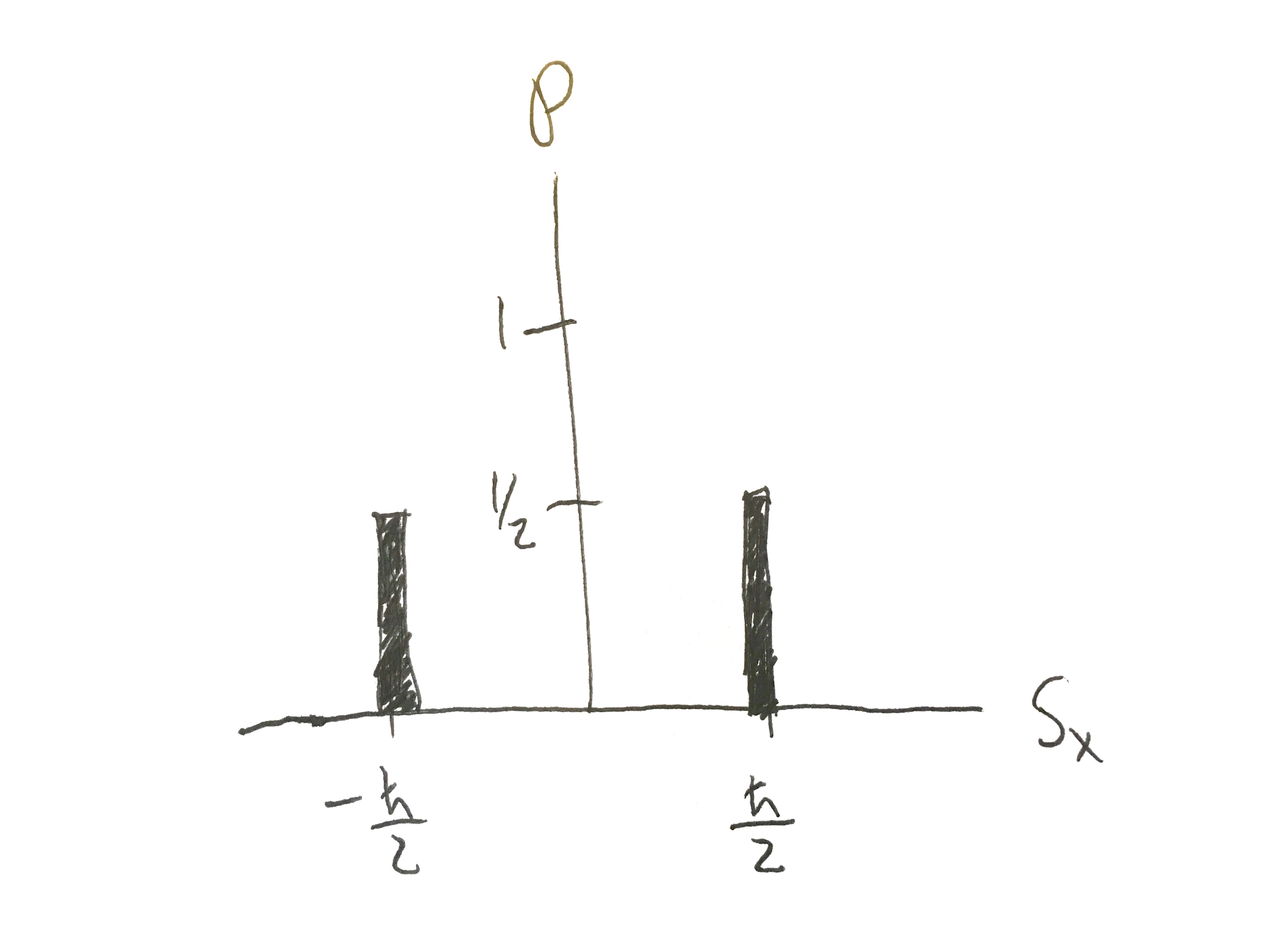
This is the \(\left|{+}\right\rangle _x\) coefficient in the expansion of \(\left|{\psi}\right\rangle \) in the \(\left|{\pm}\right\rangle _x\) basis. The probability of a measuring the \(S_x\) spin component to be \(\frac{\hbar}{2}\) is the norm squared of this coefficient. \begin{align*} \mathcal{P}({S_x = \frac{\hbar}{2}}) =& \left( \frac{2}{\sqrt{26}} - \frac{3\,i}{\sqrt{26}} \right) \, \left( \frac{2}{\sqrt{26}} + \frac{3\,i}{\sqrt{26}} \right)\\ \, =& \, \frac{4}{26} + \frac{9}{26} \\ =& \, \frac{1}{2} \end{align*} The \(\mathcal{P}({S_x = -\frac{\hbar}{2}})\) is calculated the same way (or you can subtract \(\mathcal{P}({S_x = -\frac{\hbar}{2}})\) from 1) and is \(1/2\).
- Use Another Representation: Plot histograms of the predicted measurement results from parts \((a)\) and \((b)\). Your histogram should be a vertical bar chart with the value of the spin component on the horizontal axis and the probability on the vertical axis.
For part (a):
 For part (b):
- What are the possible measurement values if you measure the spin component \(S_z\), and with what probabilities would they occur? Check Beasts: Check that you have the right “beast.”
- Phase 2
S1 5416S
Consider the three quantum states:
\[\left\vert \psi_1\right\rangle = \frac{4}{5}\left\vert +\right\rangle+ i\frac{3}{5} \left\vert -\right\rangle\]
\[\left\vert \psi_2\right\rangle = \frac{4}{5}\left\vert +\right\rangle- i\frac{3}{5} \left\vert -\right\rangle\]
\[\left\vert \psi_3\right\rangle = -\frac{4}{5}\left\vert +\right\rangle+ i\frac{3}{5} \left\vert -\right\rangle\]
- For each quantum state \(\left|{\psi_i}\right\rangle \) given above, calculate the probabilities of obtaining \(+\frac{\hbar}{2}\) and \(-\frac{\hbar}{2}\) when measuring the spin component along the \(x\)-, \(y\)-, and \(z\)-axes (i.e.,\(S_x\), \(S_x\), and \(S_z\) ).
First, you should check that the states are normalized. You can do this by taking the braket of each \(\psi\) with itself to see if you get 1. These states are normalized. The probability to end up in an state \(\left|{a_i}\right\rangle \) is given by \(\left|\left\langle {a_i}\middle|{\psi_i}\right\rangle \right|^2\). The states \(\left|{\psi_i}\right\rangle \) are given in the \(\,\widehat{\!S}_z\) basis, so probabilities for measurements of the \(z\) component of spin are practically read off: For \(\left|{\psi_1}\right\rangle \): \[ \mathcal{P}(S_z = \frac{\hbar}{2}) = \left|\left\langle {+}\middle|{\psi_i}\right\rangle \right|^2 = \left( \frac{4}{5}\right)^2 = 16/25, \]\[ \mathcal{P}(S_z = \frac{-\hbar}{2}) = \left|\left\langle {-}\middle|{\psi_i}\right\rangle \right|^2 = \left( -i\,\frac{3}{5} \right) \left( i\,\frac{ 3}{5} \right) = 9/25. \] Other probabilities are a little more interesting, and here we deal in detail with those related to the measurements of \(\,\widehat{\!S}_y\). Following the general prescription, with \(\left|{\pm}\right\rangle _y = \frac{1}{\sqrt{2}} \big( \left|{+}\right\rangle \pm i\left|{-}\right\rangle \big)\), (don't forget to complex conjugate the coefficients when taking the bra!) \begin{eqnarray*} & \displaystyle {}_y\left\langle {+}\middle|{\psi_1}\right\rangle = \frac{1}{\sqrt{2}} \bigg( \left\langle {+}\right| - i\left\langle {-}\right| \bigg) \left( \frac{4}{5}\, \left|{+}\right\rangle + i\,\frac{3}{5}\, \left|{-}\right\rangle \right) = \frac{4}{5\sqrt{2}} - \big( i \big) \left( i \frac{3 }{5\sqrt{2}} \right) = \frac{7}{5\sqrt{2}}, \\ & \displaystyle {}_y\left\langle {-}\middle|{\psi_1}\right\rangle = \frac{1}{\sqrt{2}} \bigg( \left\langle {+}\right| + i\left\langle {-}\right| \bigg) \left( \frac{4}{5}\, \left|{+}\right\rangle + i\,\frac{3}{5}\, \left|{-}\right\rangle \right) = \frac{4}{5\sqrt{2}} + \big( i \big) \left( i \frac{3 }{5\sqrt{2}} \right) = \frac{1}{5\sqrt{2}}. \end{eqnarray*} The probabilities are the squares of the norms of these coefficients, \(\mathcal{P}(S_y = \frac{\hbar}{2}) = 49/50\) and \(\mathcal{P}(S_y = \frac{-\hbar}{2}) = 1/50\) (adding up to \(1\)).
For \(\left|{\psi_2}\right\rangle \), the sign of \(i\) in the second parenthesis above is changed to minus, and we get \[ {}_y\left\langle {+}\middle|{\psi_2}\right\rangle = \frac{4}{5\sqrt{2}} + \frac{ \big(i\big) 3\,i }{5\sqrt{2}} = \frac{1}{5\sqrt{2}},\mathrm{and} {}_y\left\langle {-}\middle|{\psi_2}\right\rangle = \ \cdots \ = \frac{7}{5\sqrt{2}}. \] Note that the coefficients, and thus probabilities, are swapped compared to the previous ones; now \(\mathcal{P}(S_y = \frac{\hbar}{2})\) is \(1/50\), and \(\mathcal{P}(S_y = \frac{-\hbar}{2})\) is \(49/50\).
For \(\left|{\psi_3}\right\rangle \): \begin{eqnarray*} & \displaystyle {}_y\left\langle {+}\middle|{\psi_3}\right\rangle = \frac{1}{\sqrt{2}} \bigg( \left\langle {+}\right| - i\left\langle {-}\right| \bigg) \left( - \frac{4}{5}\, \left|{+}\right\rangle + i\,\frac{3}{5}\, \left|{-}\right\rangle \right) = - \frac{4}{5\sqrt{2}} - \frac{ \big(i\big) 3\,i }{5\sqrt{2}} = \frac{-1}{5\sqrt{2}}, \\ & \displaystyle {}_y\left\langle {-}\middle|{\psi_3}\right\rangle = \frac{1}{\sqrt{2}} \bigg( \left\langle {+}\right| + i\left\langle {-}\right| \bigg) \left( - \frac{4}{5}\, \left|{+}\right\rangle + i\,\frac{3}{5}\, \left|{-}\right\rangle \right) = - \frac{4}{5\sqrt{2}} + \frac{\big(i\big) 3\,i }{5\sqrt{2}} = \frac{-7}{5\sqrt{2}}. \end{eqnarray*} The probabilities are the same as those when the system is measured in the state \(\left|{\psi_2}\right\rangle \), above.
The calculations for \(\,\widehat{\!S}_x\) are carried out exactly the same way.
- Look For a Pattern (and Generalize): Use your results from \((a)\) to comment on the importance of the overall phase and of the relative phases of the quantum state vector.
Notice that the \(\left|{\psi_3}\right\rangle =-\left|{\psi_2}\right\rangle =e^{i\pi}\left|{\psi_2}\right\rangle \), i.e. these states differ only by an overall phase. As expected, these states are physically the same and therefore all of the probabilities that we calculated for these two states are the same. Now let us observe the relative phases between the components of these states. With phases of components written out explicitly, \[\left|{\psi_1}\right\rangle =e^{i\,0} \left|{+}\right\rangle + e^{i\,\frac{\pi}{2}} \left|{-}\right\rangle (\mathrm{since}\ e^{i\frac{\pi}{2}}= i,e^{i\,0}= 1),\] while for the other two states we have \[\left|{\psi_2}\right\rangle =e^{i\,0} \left|{+}\right\rangle + e^{-i\,\frac{\pi}{2}} \left|{-}\right\rangle ,\left|{\psi_3}\right\rangle =e^{i\,\pi} \left|{+}\right\rangle + e^{i\,\frac{\pi}{2}} \left|{-}\right\rangle = e^{i\,\pi} \Big( e^{i\,0}\left|{+}\right\rangle + e^{-i\,\frac{\pi}{2}} \left|{-}\right\rangle \Big).\] The difference between phases of the components, the “relative phase,” for \(\left|{\psi_1}\right\rangle \) is \(-\frac{\pi}{2}\), while for \(\left|{\psi_2}\right\rangle \) (and \(\left|{\psi_3}\right\rangle \)) it is \(\frac{\pi}{2}\). States that have different relative phases, like \(\left|{\psi_1}\right\rangle \) vs. \(\left|{\psi_2}\right\rangle \) (or vs. \(\left|{\psi_3}\right\rangle \)) have different probabilities. These states are physically inequivalent. Note, however, that since the coefficients in the \(z\)-basis have the same norms squared, the probabilities for spin up and spin down in the \(z\)-orientation are the same for all three states. It is not until we calculate probabilities in the \(x\)- or \(y\)-orientations that we see the inequivalence of the first state from the other two.
- For each quantum state \(\left|{\psi_i}\right\rangle \) given above, calculate the probabilities of obtaining \(+\frac{\hbar}{2}\) and \(-\frac{\hbar}{2}\) when measuring the spin component along the \(x\)-, \(y\)-, and \(z\)-axes (i.e.,\(S_x\), \(S_x\), and \(S_z\) ).
- Phase in Quantum States
S1 5416S
In quantum mechanics, it turns out that the overall phase for a state does not have any physical significance. Therefore, you will need to become quick at rearranging the phase of various states. For each of the vectors listed below, rewrite the vector as an overall complex phase times a new vector whose first component is real and positive. \[\left|D\right\rangle\doteq \begin{pmatrix} 7e^{i\frac{\pi}{6}}\\ 3e^{i\frac{\pi}{2}}\\ -1\\ \end{pmatrix}\\ \left|E\right\rangle\doteq \begin{pmatrix} i\\ 4\\ \end{pmatrix}\\ \left|F\right\rangle\doteq \begin{pmatrix} 2+2i\\ 3-4i\\ \end{pmatrix} \]
One must factor the complex exponential phase of the top component from every component of the vector.
\begin{align*} \left|D\right\rangle&\doteq \left( \begin{matrix} 7e^{i\frac{\pi}{6}}\\ 3e^{i\frac{\pi}{2}}\\ -1 \end{matrix}\right)\\ &= e^{i\frac{\pi}{6}}\left( \begin{matrix} 7\\ 3e^{i\frac{\pi}{2}}e^{-i\frac{\pi}{6}}\\ -1e^{-i\frac{\pi}{6}} \end{matrix}\right)\\ &= e^{i\frac{\pi}{6}}\left( \begin{matrix} 7\\ 3e^{i\frac{\pi}{3}}\\ -1e^{-i\frac{\pi}{6}} \end{matrix}\right)\\ \left|E\right\rangle &\doteq \left( \begin{matrix} i\\ 4\\ \end{matrix} \right)\\ &=\left( \begin{matrix} e^{i\frac{\pi}{2}}\\ 4 \end{matrix} \right)\\ &=e^{i\frac{\pi}{2}}\left( \begin{matrix} 1\\ 4e^{-i\frac{\pi}{2}} \end{matrix} \right)\\ \left|F\right\rangle &\doteq \left( \begin{matrix} 2+2i\\ 3-4i \end{matrix} \right)\\ &=\left( \begin{matrix} \sqrt{8}e^{i\frac{\pi}{4}}\\ 5e^{-0.93i} \end{matrix} \right)\\ &=e^{i\frac{\pi}{4}}\left( \begin{matrix} \sqrt{8}\\ 5e^{-0.93i}e^{-i\frac{\pi}{4}} \end{matrix} \right)\\ &=e^{i\frac{\pi}{4}}\left( \begin{matrix} \sqrt{8}\\ 5e^{-1.7i} \end{matrix} \right) \end{align*}