Oscillations and Waves: Spring-2025 HW 5b (SOLUTION): Due W5 D5
Coaxial Cable Lab Circuit Diagram
S1 5219S
Draw a schematic diagram that shows the circuit you studied in the “coaxial cable lab” on Tuesday.
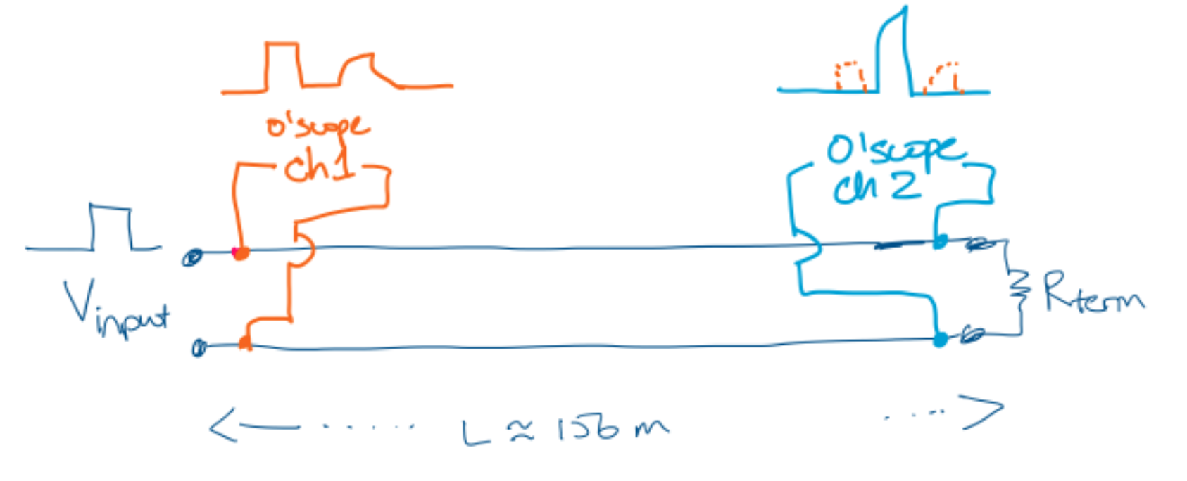
Figure: Circuit diagram of the coaxial cable, showing input pulse, terminating resistance (variable), and oscilloscope connections at both ends of the cable. The cable length is \(L\), about \(156\, m\).
Create a good caption that shows the lessons learned from the previous lab. The caption is descriptive, succinct and allows the figure and caption to stand alone.
We look forward to reading your captions!
Write a short paragraph that describes what you measured and how you measured it, referring to the diagram.
A square voltage pulse of height approximately \(2.8\,V\) is launched at one end of a coaxial cable (the “top”) as shown in the figure. The other end (the “bottom”) is terminated with a resistor \(R_{term}\), that varies from \(0\,W\) to \(600\, W\). A high-impedance oscilloscope measures the voltages at the top and the bottom. The pulse period in approximately \(\frac{1}{40}\,kHz = 25 \mu s\), and the duration is approximately \(2\)% of \(25\,\mu s\) or \(0.5\,\mu s\). The pulse time of travel is about \(1.6 \,\mu s\), so this choice allows resolution of the input and reflected pulses. As the terminating resistance changes, mimicking a second cable of different impedance, the heights of the two pulses change accordingly. The oscilloscope trace is shown in \(Q3\), the data in \(Q\)4, and a graph in \(Q5\).
Speed of Wave Propagation in a Cable
S1 5219S
Explain how you measured the speed of wave propagation in the coaxial cable.
Drive on end of the cable with a voltage pulse and see the pulse reflected from the end. On the oscilloscope, there is a time delay between the leading edge of the input pulse and the reflected pulse. Measure that time. It is generally about microseconds. The cable length is given on the spool.
What is the speed of propagation in \(m/s\)? As a fraction of the speed of light?
For my \(RG58\) cable (which was \(156\, m\) long) the time to travel \(2 x 156 = 318\,m\) was \(1.6\,\mu s\). Hence \(v= \frac{318\, m}{1.6\times 10^{-6}\,s} = 1.95\times 10^8\,m/s\) or about \(2/3\) of \(c\).
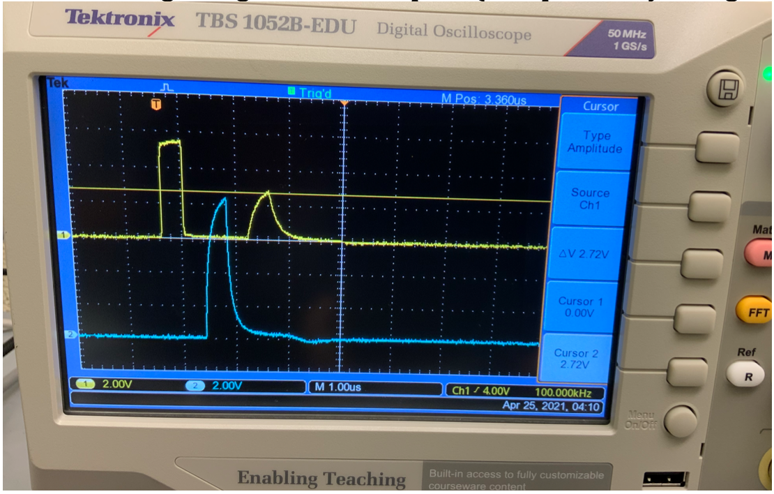
Yellow trace in above represents voltage at the input end, and blue trace at the opposite end. Note the pulse has traveled half the distance in half the time.
Are the electrons in the wires traveling at this speed? Or is their material velocity smaller? Larger?
The electrons travel locally at much more modest speeds (order of \(km/s\)), but the propagation of the information about crests and troughs is much faster. It's like a sound wave, where the air molecules vibrate a little around their equilibrium.
Coaxial Cable Lab: Data Table
S1 5219S
Create a well-organized table with a caption that records the measurements you obtained in the “coaxial cable lab”.
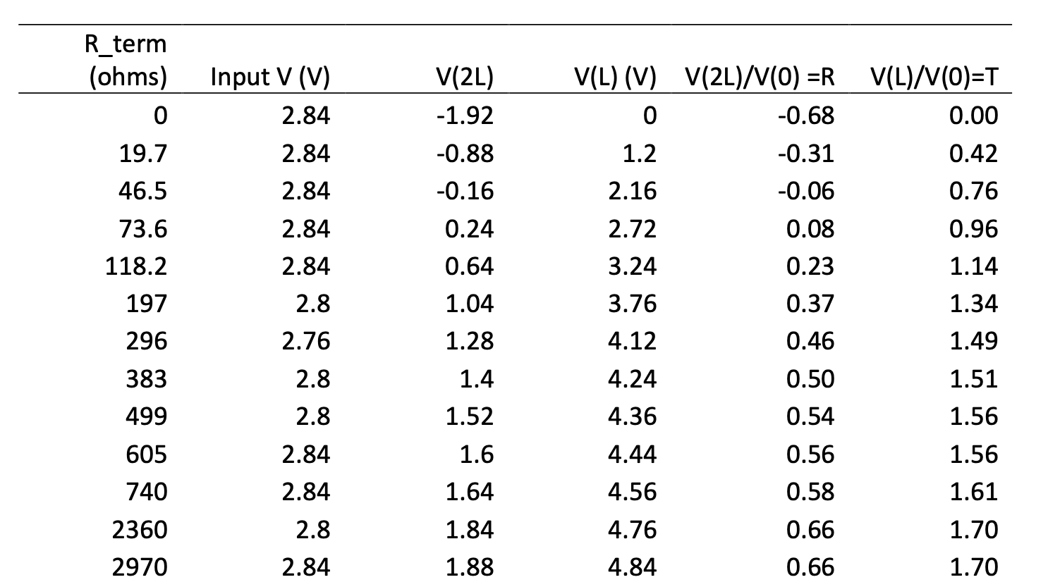
Table: Height of the voltage pulse applied (input), reflected (at \(2L\)) and transmitted (\(L\)) for each terminating resistance. The cable has length \(L\).
List the features you paid attention to when you created the table.
Your table should have
clearly labeled columns with units
appropriate significant figures
organized with like quantities grouped, or some other logical constructions
properly aligned numbers
a caption
not too busy
Coaxial Cable Lab: Graph of Voltage Ratios
S1 5219S
Plot on the same graph: (i) the height of the voltage pulse after it has propagated to the end of cable as a function of the terminating resistance and (ii) the height of the voltage pulse after it returns to the beginning of the cable as a function of the terminating resistance. Both voltages should be measured relative to the height of the pulse at the start.
Add to the plot the model for the reflection and transmission coefficients derived in class, with \(k_2\rightarrow Z_2\) representing the varying terminating resistor (“impedance of cable \(2\)”) and \(k_1\rightarrow Z_1\), representing the fixed impedance of the coax cable to be determined from your data.
My data:
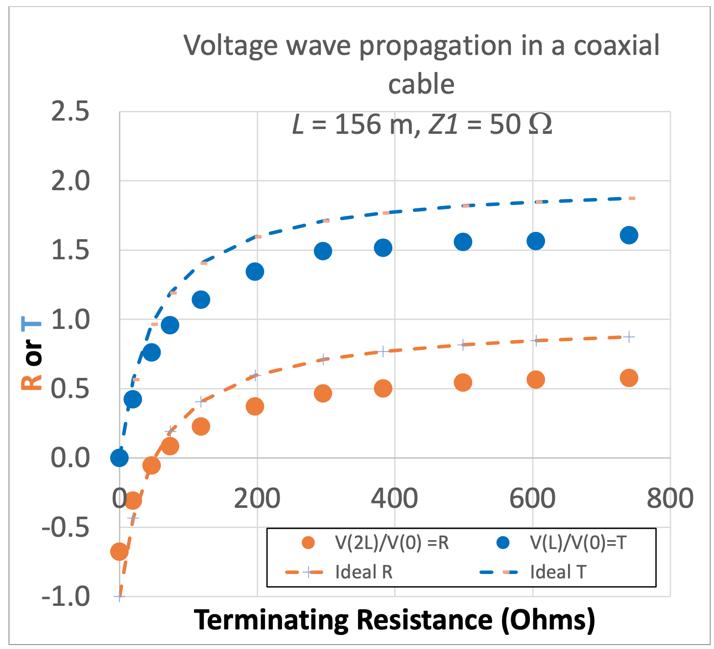
Figure: Height of the voltage pulse (relative to applied pulse height) after it has propagated to the end of cable (blue) and upon return to the top of the cable (orange) as a function of the terminating resistance.
There is a further element of the model still missing\(\dots\) what do your data suggest that the missing element is?)
The pulse height is consistently lower than predicted by the model. This suggests some loss of amplitude due to resistance which does not appear in the ideal model.
Reflection from the End of a Coaxial Cable
S1 5219S
Regarding the coaxial cable we investigated:
What is the impedance of your cable as measured by the matching terminating resistance?
For my cable, the resistance at which the reflection went to zero was \(50\,\Omega\). There were different cables. The most common impedances are \(50\,\Omega\) , \(75\,\Omega\) , \(90\,\Omega\) . You don't need to have this particular resistance as part of the set you measured --- you can interpolate between the resistances that gave the closest to zero reflection. If you're inclined, you could actually do a fit of your data to the expression we derived.
What is the total measured resistance of your cable (Be sure to include the center wire AND the shield resistances)?
For my cable, the total resistance was \(7\,\Omega \text{(center wire)} + 5.4\,\Omega \text{(shield)} = 12.4\,\Omega\).
Some cables have higher resistances, up to about \(20\,\Omega\), but usually not as high as \(100\,\Omega\). In (d), we'll need the resistance per unit length, which for my cable was \(156\,m\).
The damping parameter in \(\psi(x,t)=Re\Big[Ae^{-\frac{\Gamma}{2v} x}e^{i(\omega t \pm Kx+\phi)}\Big]\) is:
\[\frac{\Gamma}{2v}=\frac{R_0}{2L_0v}=\frac{R_0}{2L_0}\sqrt{L_0C_0}=\frac{R_0}{2}\sqrt{\frac{C_0}{L_0}}=\frac{R_0}{2Z}=\frac{0.079}{100}\frac{1}{m}\approx0.001\frac{1}{m} \]
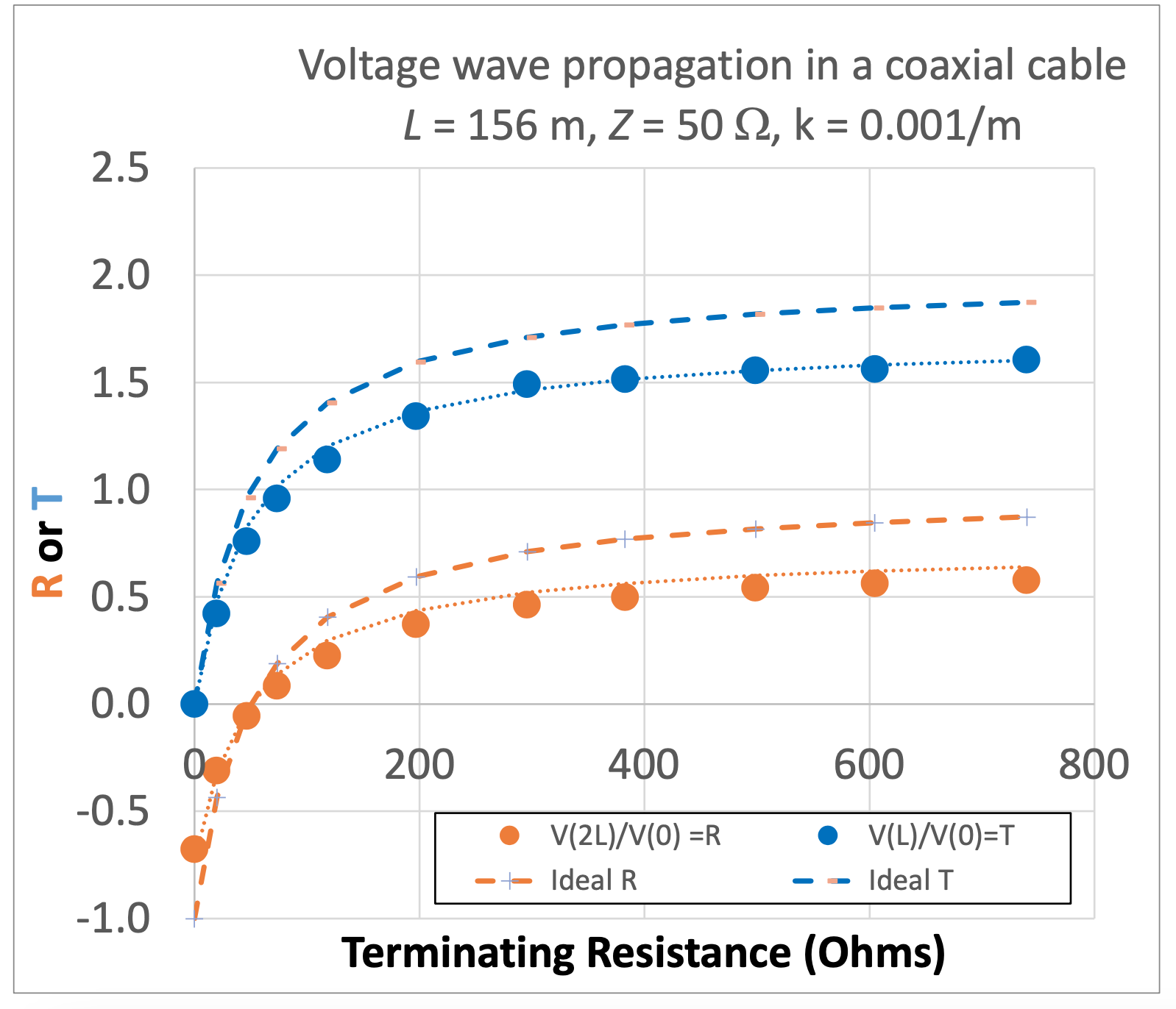
Now add to your data plot the results (use a line to indicate a model) expected from a model (i) in which resistance in the cable is neglected and (ii) resistance in the cable is incorporated and assumed to be relatively small compared to the impedance of the cable (“light damping”).
Make sure axes are properly labeled, color is nicely used to convey maximum information, and legends etc. are arranged so the reader is given the information in the clearest and most direct way.
We can multiply our theory curves by the attentuation \(e^{-\frac{\Gamma}{2Z} x}=e^{-(0.001 \frac{1}{m}) (2*156m)}=0.73\)
Figure: updated graph from previous problem with the resistance of the cable figureed into the smaller dotted line model graph.