Oscillations and Waves: Spring-2025
HW 3b (SOLUTION): Due W3 D5

1. LRC Draft Lab Writeup S1 5214S This homework assignment is entirely geared to guiding you through the lab write-up. Anything assigned here will make an important contribution to your report. Part of the assignment addresses fundamental understanding and parts asks you to reflect on communication.

   1. Circuit Diagram

      Create a diagram with caption of the LRC circuit you investigated in Thursday's lab. It does not have to be an original creation, but if it is not, you should acknowledge the source in the caption.

      • Create a caption for your figure contains a figure number and an informative but succinct description so that the figure and caption together can stand alone. Use the captions in the McGuyer paper on the canvas website as a model.
      • What information would you want in a figure caption to understand the context? Go beyond the obvious “Circuit diagram,” but do not introduce new physics or discussion. That's for the text.
      • What features of a caption do you consider important? In the McGuyer paper on the canvas website, state one feature that you think is well done. Anything surprising to you?

   2. Figures showing driving voltage and response

      For the three cases \(\omega < \omega_0\), \(\omega = \omega_0\), \(\omega > \omega_0\) generate a figure that illustrates the circuit response relative to the driving voltage. Decide whether one graph or three is best. Provide a good caption for the figure.

   3. Table of raw and processed results

      From HW 2b, take the table you generated, and prepare a well-crafted table that has the relevant raw numbers you recorded and the derived quantities.

      • Pay attention to significant figures, column headings and units, clarity of presentation.
      • Write a caption for the table. Can the reader easily make sense of the table?

      This table could appear in the main body of your text, or it could be placed in an appendix.

   4. Graphs of \(|I(\omega_d)|\) and \(\phi_I (\omega_d)\) data and model

      Generate a graph of \(|I(\omega_d)|\) (or a quantity proportional to it that you prefer to communicate) as a function of \(\omega_d\) (or \(f_d\) if you prefer that variable) from your measured values. On the same graph, present the prediction from the model we studied in class. Is the model satisfactory? If not, what actions do you suggest?

      Repeat for the phase \(\phi_I(\omega_d)\) or \(\phi_I(f_d)\) if you prefer \(f_d\) as a variable.

      • How is the model prediction most effectively presented? Lines? Points? Different color?
      • Create a caption for these plots. Have you clearly differentiated between the model and the data in the caption?

   5. Draft

      Draft your report by creating section headings for all sections of the report. The draft should contain

      • the plots and captions you generated in 1-4,
      • the paragraphs you drafted in HW2b

      • and at least a 1-paragraph description of what you plan to put in any section where you don't have any text yet.

        This draft then will be polished into a Final Report to turn in on Tuesday of Week 4.

        We will try to get feedback to you in a timely fashion.

2. LRC Behavior At, Above, and Below Resonance S1 5214S

   You should find the Mathlet at https://mathlets.org/mathlets/series-rlc-circuit useful. In fact, the purpose of this question is really to get you to explain that simulation confidently.

   A series LRC circuit is driven by a sinusoidal voltage that by convention we write: \[|V_0|\cos{(\omega t)=Re[|V_0|e^{i\omega t}]}\]

   1. Draw phasor diagrams (i.e. on an Argand plot) representing the driving voltage at \(t=0\) and each of the voltages across teh capacitor \(V_C\), resistor \(V_R\), inductor \(V_L\) in a driven \(LRC\) circuit for three different cases: \((1) \,\omega << \omega_0\), \((2)\,\omega=\omega_0\) (resonance frequency), \((3)\,\omega>>\omega_0\). One phasor is filled in for you, with the red arrow representing the phase of the input voltage into the circuit and the blue arrow representing the phase of the voltage across the circuit component. Don't worry too much about the magnitudes of each arrow.

      

      Use the Mathlet at https://mathlets.org/mathlets/series-rlc-circuit for a good visualization and animation (check the “phasor diagram” box).
      A phasor is a representation of a complex number on the Argand plane. Below, the voltages are drawn as phasors at a particular time. A red phasor represents the applied voltage (along the real axis by convention) and the blue phasor is voltage across the relevant circuit element. These diagrams attempt to represent the absolute voltage magnitudes correctly e.g. at resonance, \(V_R = V_{ext}\), but the direction is emphasized here.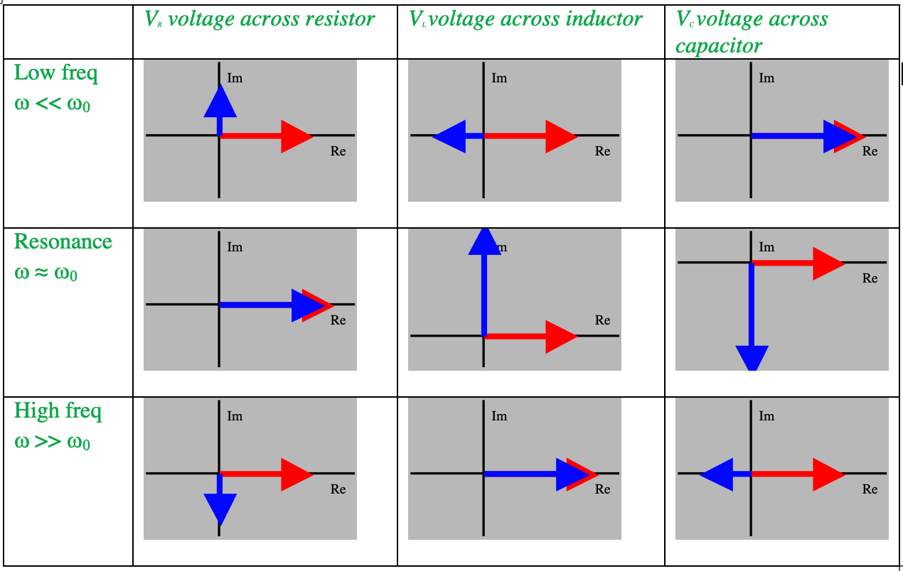

      

   2. Can you explain why we say the circuit is predominantly resistive at resonance, predominantly capacitative at low frequencies, and predominately inductive at high frequencies?

      An inductor's response to an alternating current or AC applied voltage is to reduce the flow of current, but its response is proportional to the rate of change of current. At high frequencies, the current changes from max to min very fast. Thus at high frequency, an inductor is the most important element -- it is the current limiter -- and the voltage across the inductor dominates. At low frequency, when the rate of current change from max to min is slow, the effect of the inductor is negligible. It behaves as a piece of wire.

      The capacitor's ability to allow passage of AC current depends on the speed with which the electric field between the plates changes. At low frequencies, the time rate of change of current is small, and the capacitor acts as an open circuit. The capacitor is the current limiter. At high frequencies, the capacitor offers essentially no hindrance to current flow, and is negligible.

      The frequency that divides “high” from “low” is called the resonance frequency, and at this frequency, the voltages across \(L\) and \(C\), although fairly large, exactly cancel one another, and all the applied voltage appears across the resistor. Thus the circuit is “resistive”.

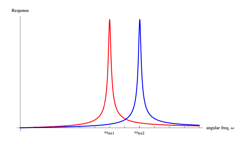
3. Broadcast Bandwidth S1 5214S FM radio stations have broadcast frequencies of approximately \(100\,MHz\). Assume that your radio uses a series LRC circuit similar to the one you used in the lab as part of the receiver electronics. The quality factor \(Q\) of the receiver circuit determines the spacing of the broadcast frequencies of the stations your receiver pick up without interference from other stations. Estimate the spacing of the broadcast frequencies of FM stations if typical receivers have a \(Q\) of \(500\) or better. Explain your reasoning, and include a graph to illustrate (sketch is OK).

   The \(Q\) factor of a circuit is determined by \(Q\equiv\frac{\omega_0}{\Delta\omega}=\frac{f_0}{\Delta f}\), where \(f_0\) is the center frequency and \(\Delta f\) is the full width at half maximum of the power or energy response. One assumes that the centers of response curves must be separated by at least \(\Delta f\) to be “resolvable” (see graph for qualitative idea). Then \(Q=\frac{f_0}{\Delta f}=500\) and \(\Delta f=\frac{f_0}{Q}=\frac{100\,MHz}{500}=0.2\,MHz\). The frequency spacing must be about \(200\,kHz\) and this would correspond to stations broadcasting at \(99.1\,MHz\), \(99.3\,MHz\), etc.. If you are tuned to the lower resonance frequency, you will pick up signals at frequencies higher too, but with lower amplitude. If another station is broadcasting at one of those higher frequencies, you'll pick that up too (at low amplitude), and it will interfere. You have to decide what constitutes acceptable interference. Of course, the higher the \(Q\) (i.e. the narrower the response curve), the more high and low frequencies the circuit will “reject”.