Oscillations and Waves: Spring-2025 HW 3a (SOLUTION): Due W3 D2
LRC Lab: Draft Experimental Setup
S1 5213S
Write \(1-2\) paragraphs that describe what measurements you made in the lab on Thursday. You should include a circuit diagram, and explain the function generator and oscilloscope.
The main idea was to “get words on paper". Most problems with writing reports arise because people are afraid to write anything for fear of imperfection, that it is not “what the teacher wants," or they simply do not know what to say. Once you have the words written, it's easier to edit. A description of the methods should not read like a lab manual with instructions to “do this, do that."
Start by describing the circuit: “A circuit with inductance \(L=XX\,mH\), capacitance \(C=XX\,nF\), etc., is connected in series and driven by a sinusoidal voltage with amplitude \(2\,V\) as shown in Fig. \(1\)" (and of course there should be a Fig. 1 with a nice informative caption).
You should explain what voltages were measured and how and why. You could then describe what the traces look like, the voltage across the resistor is also sinusoidal with the same frequency, and is phase shifted. You notice that as the frequency is changed, the amplitude and phase also change and you recorded these changes for frequencies from \(xx\) to \(yy\,Hz\). And so on ... you tell the story.
LRC Draft Lab Results
S1 5213S
Show a plot (or at least a screenshot, though your report will need actual data and not a screenshot) of the oscilloscope traces to demonstrate the external voltage driving the series LRC circuit and the voltage across the resistor in the three cases \(\omega<\omega_0\), \(\omega\approx\omega_0\) and \(\omega>\omega_0\). Write sentences describing the waveforms and indicate where you measured the amplitudes and relative phases.
You might think that it is a simple matter to simply dump some screenshots and let readers look for themselves. But you might remember that when you first looked at the screens, you had to have it explained to you that the two traces had the same frequency (as the model predicted) and that one was a scaled, phase shifted version of the other. To make a really compelling figure, consider exporting the raw data (right click and export to Excel) and creating a clean, clear plot in Excel.
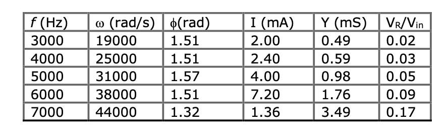
Make a table displaying the relevant voltages you measured and the time (and phase) differences you observed for the appropriate range of frequencies. Organize your table clearly, and make sure that columns are titled, with units given. Even if you haven't finished the measurements, you should still have a plan to organize the measurements in a well-constructed table.
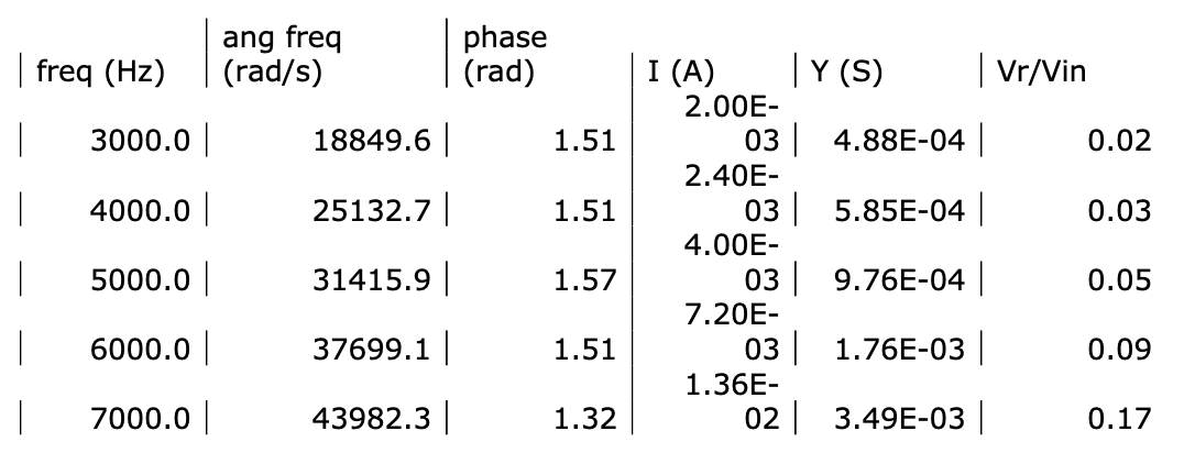
Good tables are an art. Representative rather than compreshensive data would be helpful. Here's a bad table:
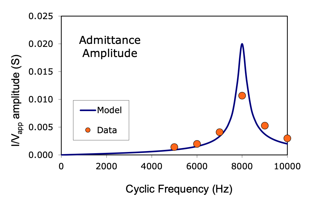
If you have any data, make a plot of the amplitude of the current in the circuit (per unit voltage applied) i.e. admittance, as a function of frequency. Also plot the relative phase as a function of frequency. Reflect on your results.
Here's an example of data points superimposed on a model. You may not be at this point yet, but you should get there. Just having data is good. Setting it up against a model is the next most important step. Formatting comes next. If the plot is compelling, what features make it so? How can you improve this presentation?
This plot was generated in Excel, so Excel can be forced to produce good-looking plots. It takes some effort, though. You may have better plotting software at your disposal. However, Excel is extremely convenient for modeling data and changing things on the fly.
Q factor of a Resonance Circuit
S1 5213S
We define a “quality factor”, \(Q\equiv\frac{\omega_0}{2\beta}\), and use it as a measure of cycles in a free (undriven), damped oscillator before the oscillation decays to some smaller amplitude. The larger the number of cycles, the larger the \(Q\). Now let's see what this quantity translates to in a driven, damped oscillator. Use the example of charge amplitude\(|q|\) for a series LRC circuit.
Show that at both frequencies \(\omega=\omega_0 +\beta\) and \(\omega=\omega_0-\beta\), the magnitude of the charge response \(|q|\) is \(\frac{|q|_{max}}{\sqrt{2}}\).
(Hint -- this is a 3-line calculation. You don't need the definition of \(|q|\) in terms of \(L,\,R,\,C\)).
The definition of \(\omega_+\equiv\omega_0+\beta\) is \(\frac{E(\omega_+)}{E_{max}}=\frac{1}{2}\)
Because \(E=\frac{|q|^2}{2C}\), it follows that \(\frac{|q|^2(\omega_+)/2C}{|q|^2_{max}/2C}=\frac{1}{2}\)
Cancel terms and take the square root, \(\frac{|q|(\omega_+)}{|q|_{max}}=\frac{1}{\sqrt{2}}\)]]
Same argument for \(\omega_-\equiv\omega_0-\beta\)
At these frequencies, how large is the energy in the capacitor compared to the maximal energy at \(\omega\approx\omega_0\)?
The energy in a capacitor is proportional the the charge squared, so at those frequencies, the energy is half its value compared to at resonance.
Given the above, operationally, how would you measure the \(Q\) of a resonant circuit? What is \(Q\) for your circuit?
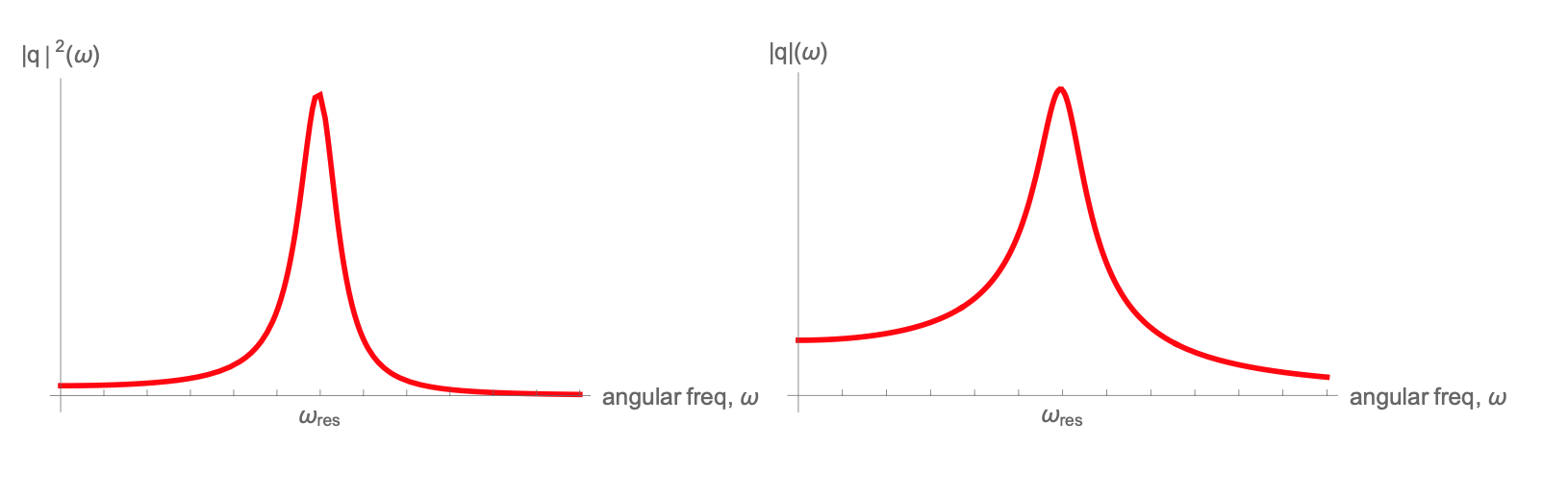
You didn't measure \(|q|\), you measured \(|dq/dt|\), but it is proportional to \(|q|\), so find the frequencies where the value of \(|dq/dt|\) falls to \(\frac{1}{\sqrt2}\approx0.7\) of its maximum value. (At these frequenciees, the value of \(|q|^2\) drop to \(\frac{1}{2}\) its maximum value, and hence defines \(Q\)). Find the difference between those two values. That difference corresponds to the FWHM of the energy curve. That is, if you'd plotted \(|q|^2\) and found the frequencies where \(|q|^2\) drop to \(\frac{1}{2}\) its maximum value, you'd get the same result.
For your circuit, \(Q\approx20\)
The graphs below may help with a visual feel for the quantities discussed above:
Steady State Solutions for the LRC Circuit
S1 5213S
Write the equation of motion governing the charge on the capacitor in a series LRC circuit driven by an external sinusoidal voltage. Identify all parameters in your equation.
The equation is found from adding thet voltages across the inductor, capacitor, and resistor and setting them equal to the driving voltage: \(V_C+V_L+V_R=V_{ext}\), where \(V_C=\frac{q}{C}\,(q=\) charge and \(C=\) capacitance), \(V_R=IR \,(I=\frac{dq}{dt}=\) current, \(R=\) resistance), and \(V_L=L\frac{dI}{dt}\,(L=\) inductance), \(V_0\) is the amplitude of the external driving voltage. Define \(\frac{1}{LC}\equiv\omega_0^2\); \(\frac{R}{L}\equiv2\beta\) and obtain:
Find a steady-state solution (or particular solution) for the current in the circuit. After what time is the steady state the only relevant part of the solution, i.e., after what time has the transient solution decayed for the circuit you are working with?
The steady state solution is the particular solution. It becomes the only part of the solution after the time longer than \(1/\beta\), when the transient has decayed away. Make the ansatz that \(q(t)=|q|e^{i\phi_q}e^{i\omega t}\) where \(|q|\) is a real number that is the amplitud of the charrge oscillations and \(\phi_q\) is the phase relative to the driving voltage, and substitute:
\[-\omega^2|q|e^{i(\omega t +\phi_q)}+2\beta i \omega|q|e^{i(\omega t+\phi_q)}+\omega_0^2|q|e^{i(\omega t+\phi_q)}=\frac{V_0e^{i\omega t}}{L}\]
Cancel the time dependence, which proves the ansatz works. Solve for the unknowns:
\[|q|e^{i\phi_q}=\frac{V_0/L}{(-\omega^2+2\beta i\omega+\omega_0^2)} \]
Rewrite the right-hand side in polar form (class exercise):
\[|q|e^{i\phi_q}=\frac{V_0/L}{\sqrt{{(\omega_0^2-\omega^2)+(2\beta\omega)^2}}}e^{-i\theta} \]
where \(\tan{\theta}=\frac{2\beta\omega}{\omega_0^2-\omega^2}\). Identify the magnitudes and phases:
\[|q|=\frac{V_0/L}{\sqrt{(\omega_0^2-\omega^2)+(2\beta\omega)^2}}\]
\[\tan{\phi_q}=\frac{-2\beta\omega}{\omega_0^2-\omega^2}\]
Differentiate to find current:
\[I(t)=\dot{q}(t)=i\omega q(t)=\omega e^{i\pi/2}q(t)\]
so we can write current in the form
\[I(t)=Re[|I|e^{i(\omega t+\phi_I)}]\]
with
\[|I|=\omega|q|=\frac{\omega V_0/L}{\sqrt{(\omega_0^2-\omega^2)^2+(2\beta\omega)^2}}\]
\[\phi_I=\frac{\pi}{2}+\phi_q\]
Find the steady state solution for \(\frac{dI}{dt}\) in this circuit.
Differentiate to find \(\frac{dI}{dt}\): \(\dot{I}(t)=\ddot{q}(t)=-\omega^2q(t)=\omega^2e^{i\pi}q(t)\)
So we can rewrite the derivative in this form: \(\dot{I}(t)=Re[\,|\dot{I}|\,e^{i(\omega t+\phi_{\dot{I}})}]\) with
\[|\dot{I}|=\frac{\omega^2 V_0/L}{\sqrt{{(\omega_0^2-\omega^2)+(2\beta\omega)^2}}}\]
\[\phi_{\dot{I}}=\pi+\phi_q\]