Oscillations and Waves: Spring-2025
HW 2b (SOLUTION): Due W2 D5
- A Physical System that Oscillates
S1 5212S
A mass \(m\) is strung on a very light wire equidistant between two anchor points separated by a distance \(2L\). When the mass is displaced laterally (i.e. plucked) in the \(x\)-direction (here vertically), there is constant tension \(T\) on the wire that produces a restoring force.
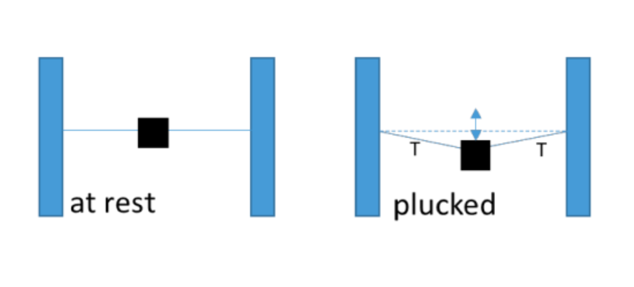
What is the resulting natural frequency \(\omega_0\) of the oscillating mass? Assume tension drives the oscillation (i.e. no gravity) and assume the angle the string makes with the posts is small.
Note: \(\omega_0\) must be expressed in terms of the physical parameters given in the problem (\(T, L, m\)).
- Write a generic expression for displacement from equilibrium in any of the standard forms, \(ABCD\).
The goal here is to `make your system look like the mass-spring system'! In other words, try to find the force in the form:
\[F=(minus)(some\,constant)\cdot(displacement)\]
If you can do that, then you can identify \((some\,constant)\) with the spring constant \(k\), and divide it by the known mass \(m\) to find the frequency.
Each wire segment has a tension \(T\) and makes an angle \(\theta\) with its respective anchor point. Therefore, the restoring force for each wire segment is the vertical component of the tension \((T\sin{\theta})\), and the total restoring force (magnitude) is \[|F_{res}|=2T\sin{\theta}\approx 2T\theta\] if the angle is small. Note the correct units. \(T\), the tension, is a force.
The restoring force points upward when the displacement is downwards, and vice versa (it would point downward if the displacement is upwards).
Further, to express everything in terms of \(x\), we note \(x=L\tan\theta\approx L\sin\theta\approx L\theta\) to the same order of approximation.
\[F_{res}\approx -2T\frac{x}{L}\]
if the angle is small, and the negative sign properly accounts for direction.
The restoring force is therefore of the form of Hooke's Law: \(F_{res}\approx-kx\) and the role of \(k\) is played by \(2\frac{T}{L}\)!
Hence, the natural frequency is \(\omega_0=\sqrt{\frac{2T}{mL}}\), where \(m\) is the mass of the mass (naturally), and any mass of the wire is neglected because it is `very light' compared to the mass.
The equation of motion in form \(A\) is:
\[x(t)=A\cos{\left(\sqrt{\frac{2T}{mL}}\,t+\phi\right)}\]
with \(A\) and \(\phi\) determined by the initial conditions.
- Phase lead/lag
S1 5212S
Sketch on one plot, two oscillations (\(\#1\) and \(\#2\)) of the same period (\(1\,s\)), where oscillation \(\#2\) has an amplitude that is twice that of oscillation \(\#1\) and lags oscillation \(\#1\) by \(\frac{\pi}{4}\).
At time \(t = 0\), the red (\(\#1\)) oscillation is at its peak. The blue one (\(\#2\)) has not reached its peak, but will so in \(\frac{1}{8}\) of a cycle \((=\frac{\pi}{4}\times \frac{1}{2\pi})\), so it lags the red one.
We can compare phases even though the amplitudes (maximum excursions) are different. If the frequencies are different, we can still compare phases, but the phase difference does not remain constant, and one oscillation could lead, then later lag.

Sketch on one plot, the charge \[q(t) = Q \cos{(\omega_0 t)}\] and the current \[I(t) = \dot{q}(t)\] and say which one leads and by what phase. Give a verbal explanation.
Note: It is good to object to plotting \(2\) quantities with different dimensions on the same vertical axis! But it is okay if you think of the plot as having a left vertical axis for one quantity and a right axis for the other. The important thing is to get the horizontal time axis to line up for both oscillations.
\[q(t) = Q\cos{(\omega_0 t)}\] Current \begin{align*} I(t) &= \dot{q}(t) \\ &= -Q\omega_0 \sin{(\omega_0 t)} \\ &= Q\omega_0 \sin{(\omega_0 t + \pi)} \\ &= Q\omega_0 \cos{(\omega_0 t + \pi - \frac{\pi}{2})} \\ &= Q\omega_0 \cos{(\omega_0 t + \frac{\pi}{2})} \end{align*}
At time \(t=0\), the red (charge) oscillattion is at its peak. The blue one (current) has already reached its peak, \(\frac{1}{4}\) of a cycle ago, so it leads the red one.
(Note: You could argue that it lags by \(\frac{3}{4}\) of a cycle, but we confine the words “lead” and “lag” to the interval \(\pm\frac{T}{2}\).)
The amplitudes are drawn the same, but the scale is coulombs for charge and amps for current. No numbers were given in the setup, I chose some numbers for the axes labels. The important feature is the alignment of the two graphs with respect to phase and time.

- Damped Oscillator
S1 5212S
An undamped oscillator has a period \(T_1=1.000\) s, that increases to \(T_2=1.001\) s when damping is added.
What is the damping factor \(\beta\)?
Looking at the differential equation for a lightly damped oscillator,
\begin{equation*} \ddot{x}+2 \beta \dot{x}+\omega_{0}^{2} x=0 \end{equation*} I can assume a solution is in the form of \begin{equation*} x=C e^{p t} \end{equation*} and plugging \(x\left(t\right)\) into the differential equation I find an equation in which I can solve for \(p\).
\begin{equation*} \begin{array}{l}{p^{2} x+2 \beta p x+\omega_{0}^{2} x=0} \\ {p^{2}+2 \beta p+\omega_{0}^{2}=0} \\ {p=-\beta \pm \sqrt{\beta^{2}-\omega_{0}^{2}}=-\beta \pm \omega_{1}}\end{array} \end{equation*} where \begin{equation*} {(i\omega_1)}^2=-\omega_{1}^{2}=\beta^{2}-\omega_{0}^{2} \end{equation*} Now I can solve for \(\beta\). \begin{equation*} \beta=\sqrt{\omega_{0}^{2}-\omega_{1}^{2}} \end{equation*}
By what factor does the oscillation amplitude decrease after 10 cycles?
Knowing that \(T=\frac{2\pi}{\omega}\), I can find a numerical solution for \(\beta\). \begin{equation*} \beta=\sqrt{\left(\frac{2 \pi}{T_{0}}\right)^{2}-\left(\frac{2 \pi}{T_{1}}\right)^{2}}=0.281 s^{-1} \end{equation*} After 10 cycles I have the amplitude reduced by a factor of \(e^{-0.281*10}=0.06.\)
- Underdamped LRC Oscillator
S1 5212S
Consider an oscillator with capacitance \(C=18\,nF=18\times 10^{-9}\,F\), a resistor of resistance \(R=50\,\Omega\) and an inductor with an inductance \(L=22\,mH=0.022\,H\). Charge the isolated capacitor up and then connect it in series to the \(L\) and \(R\) and allow it to discharge. Assume the starting time is \(t=0\).
What are the initial conditions for this circuit?
The charge is easier (See LC oscillator question) \[q(0)=Ae^{-\beta 0}\cos{(\omega_1 0 +\phi)}=A\cos{(\phi)}\] The current is less obvious. Because of the inductor, the current in the circuit cannot hop instantaneously to a large value so (at the level of approximation where \(\beta<<\omega_1\) so the second term in the time derivative can be neglected). \[I(0)\approx A\omega_1 e^{-\beta 0}\sin{(\omega_1 0+\phi)}=A\omega_1\sin{(\phi)}=0\] Thus, \(\phi=0\) and \(q(0)=A=36\,nC\).
What is the damping time (time for amplitude to decay to \(1/e\) of starting value)?
\[q(t)=Ae^{-\beta t}\cos{(\omega_1 t+\phi)}\] The amplitude is \(Ae^{-\beta t}\) and is \(A\) at \(t=0\). At \(t=\frac{1}{\beta}\), \(|q(t=1/\beta)|=Ae^{-1}\)
The value is \(t=\frac{1}{\beta}=\frac{2L}{R}=\frac{2\times22\times10^{-3}\,H}{50\,\Omega}\approx0.9\,ms\) (or approximately \(1\,ms\))By what fraction is the oscillation frequency shifted from the undamped version?
The shifted frequency is: \(\omega_1=\sqrt{\omega_0^2-\beta^2}=\omega_0\sqrt{1-\frac{\beta^2}{\omega_0^2}}\approx\omega_0(1-\frac{\beta^2}{2\omega_0^2}+...)\) where we have used the expansion of a power and \(\beta^2 << \omega_0^2\)// So, \(\frac{\omega_1}{\omega_0}\approx(1-\frac{\beta^2}{2\omega_0^2}+...)=1-\frac{LC}{2}\times\frac{R^2}{4L^2}=1-0.00025\), which is a very small shift from 1!! You could also write \(\frac{\omega_1-\omega_0}{\omega_0}\approx0.00025\).
How many cycles occur within the damping time?
Each period is \(=0.125\,ms\) (we can use either \(\omega_0\) or \(\omega_1\) to calculate).
The damping time is \(\frac{1}{\beta}=0.9\,ms\) The number of cycles in the damping time is \(\frac{\frac{1}{\beta}}{T}=\frac{0.9\,ms}{0.125\,ms}\approx7\)What is the value of the quality factor (or Q-factor) of the circuit? Look up another system to put this Q-factor in some sort of context.
The quality factor is \(Q\equiv\frac{\omega_0}{2\beta}=\frac{2\pi}{2\beta T}=\frac{\pi(\frac{1}{\beta})}{T}\approx22\)
According to Wikipedia, https://en.wikipedia.org/wiki/Q_factor, tuning forks have \(Q\) factors of about \(1000\). So-called Q-switched lasers can have \(Q\approx10^{11}\) or higher.How long will it take for the system lose \(90\%\) of its energy?
At \(t=0\), the system has energy \(U=\frac{1}{2C}q^2\) (all the energy is in the capacitor and none in the inductor because the current is zero at that instant.) We should find the energy (amplitude) \(|U(t)|=\frac{1}{2C}A^2e^{-2\beta t}\) to decay to \(0.1\) of its starting value, which occurs when
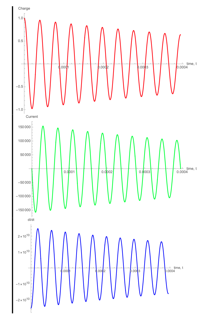
\[e^{-2\beta t}=0.1\rightarrow-2\beta t=\ln{(0.1)}\rightarrow t=\ln{(0.1)}\approx1\,ms\] Very similar to the \(1/e\) time for the charge, but there's no particular significance -- just that \(e^{-2}\approx0.1\)- Plot the charge, current, and current derivative (\(\dot{I}\)) in the circuit as functions of time for enough cycles to show the damping. Use Mathematica, Python, or the software of your choice.