Energy and Entropy: Fall-2024
HW 2 (SOLUTION): Due Day 8 Fri 10/4
- Derivatives from Data (NIST)
S1 5072S
Use the NIST web site “Thermophysical Properties of Fluid Systems” to answer the following questions. This site is an excellent resource for finding experimentally measured properties of fluids.
- Find the partial derivatives
\[\left(\frac{\partial {S}}{\partial {T}}\right)_{p}\]
\[\left(\frac{\partial {S}}{\partial {T}}\right)_{V}\]
where \(p\) is the pressure, \(V\) is the volume, \(S\) is the entropy, and \(T\) is the temperature. Please find these derivatives for one gram of methanol at one atmosphere of pressure and at room temperature. Please note, you will encounter a problem if your step in \(T\) is too small, and you will encounter a different problem if your step in \(T\) is too big.
To find the derivative for constant pressure, we need an isobaric process, and for constant volume, we need an isochoric process. So we'll need 2 sets of data from NIST. These solutions will be using the following units: Temperature (Kelvin) at 300K, and Entropy (J/K), and selecting pressure equal to 1 atm and with 1 gram of methanol, let's start with the NIST data for constant pressure. First, look at the graphs and check that they appear as linear as you need them to be. Otherwise, choose a smaller interval. After selecting processes and inputing these, I recommend downloading the data table and using points on either side of the target temperature and pressure and reducing the differentials to deltas to find the approximate derivative, but there are other methods that will give nearly the same result. \begin{align} \left(\frac{\partial S}{\partial T}\right)_P = \left(\frac{\Delta S}{\Delta T}\right)_P =\left(\frac{-9.8608 \frac{J}{mol*K}-(-10.405 \frac{J}{mol*K})}{301 K-299 K}\right)=0.544 \frac{J}{mol*K^2} \end{align} In your data table for constant temperature, you'll notice a column that gives the density of methanol. It is important to recognize that this density does not change much over a small range of temperature, so we should be able to use it for the isochoric process. In order to generate that data on NIST, we will need to input that density. Now using the data generated for an isochoric process, we get: \begin{align} \left(\frac{\partial S}{\partial T}\right)_V = \left(\frac{\Delta S}{\Delta T}\right)_V =\left(\frac{-9.9065 \frac{J}{mol*K}-(-10.401 \frac{J}{mol*K})}{301 K-299 K}\right)=0.247 \frac{J}{mol*K^2} \end{align}
- Why does it take only two variables to define the state?
The number of variables it takes define a state is equal to the number of ways there are to get energy into or out of the system. In this situation, we only have heat and work, so two variables define the state.
- Why are the derivatives above different?
Holding different variables constant and at different amounts changes how energy enters and leaves the system, and at what rate it does so. Holding a different quantity constant sends us along a different path through the thermodynamic system (because we're going through a different process! Isobaric vs. isochoric!). As such, we have different changes in our thermodynamic variables AND different changes in the slopes of these curves, which means different derivatives.
- What do the words isobaric, isothermal, and isochoric mean?
The prefix "Iso-" means to keep the same, so these are all processes that hold something constant. The suffix -Thermal indicates temperature, so Isothermal means "same temperature" or hold temperature constant. -Baric has the same origin as for Barometer, a device that measures pressure, so remember this as holding pressure constant. Finally, the suffix -Choric doesn't have an English word with the same Greek root, so it's harder to remember. Isochoric is a constant volume process, also known as an isovolumetric process or isometric process.
- Find the partial derivatives
\[\left(\frac{\partial {S}}{\partial {T}}\right)_{p}\]
\[\left(\frac{\partial {S}}{\partial {T}}\right)_{V}\]
where \(p\) is the pressure, \(V\) is the volume, \(S\) is the entropy, and \(T\) is the temperature. Please find these derivatives for one gram of methanol at one atmosphere of pressure and at room temperature. Please note, you will encounter a problem if your step in \(T\) is too small, and you will encounter a different problem if your step in \(T\) is too big.
- Translating Contours
S1 5072S
Consider the following diagram of \(T\) vs \(V\) at different \(p\). The diagram illustrates the relationship between pressure, volume and temperature for an unknown substance (do not assume this is an ideal gas).
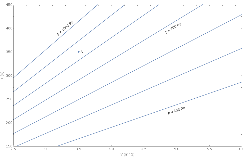
Translate the information on this diagram from the T-V plane to the p-V plane (i.e. draw contours of constant \(T\) on a graph of \(p\) vs \(V\)). Include point \(A\) on your p-V graph. Complete your graph by hand using discrete data points that you read from the T-V diagram. Make a fairly accurate sketch of the contours using the attached grid or in some other way making nice square axes with appropriate tick marks. Don't make up data for pressures above 1000 Pa or below 400 Pa.

Each dot on the graph below was obtained from the T-V diagram by drawing a horizontal line of contant \(T\) and reading off the volume associated with \(p\) = 400, 500, 600, 700, 800, 900, 1000 Pa.
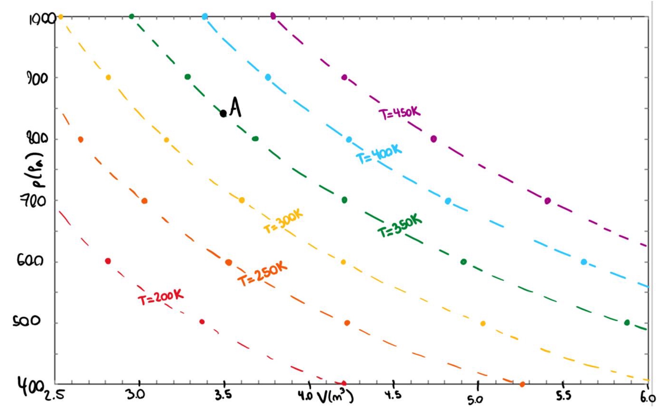
Are the lines that you drew straight or curved? What feature of the \(TV\) graph would have to change to change this result?
The lines end up curved! This relationship is not a linear one. When looking at the \(TV\) graph, the lines of constant \(p\) would have to be evenly spaced when moving horizontally (at fixed \(T\)) in order to give straight lines when we translate.
Sketch the line of constant temperature that passes through the point A.
The line of constant temperature passing through A has to be interpolated, so it is not shown on the graph. This line should have the same general shape as the surrounding lines while passing through the point A.
What are the values of all the thermodynamic variables associated with the point A?
The values at point A are approximately \(V = 3.5\) m3, \(T = 350\) K and \(p = 850\) Pa.
- Zapping With d 1
S1 5072S
Find the differential of each of the following expressions; zap each of the following with \(d\). Note that all italicized letters are variables:
\[f=3x-5z^2+2xy\]
\begin{equation*} df = 3\ dx - 10 z\ dz + 2x\ dy + 2y\ dx \end{equation*}
\[g=\frac{c^{1/2}b}{a^2}\]
\begin{equation*} dg=\frac{c^{-1/2}b}{2a^2} dc + \frac{c^{1/2}}{a^2} db -\frac{2c^{1/2}b}{a^3} da \end{equation*}
\[h=\sin^2(\omega t)\]
\begin{equation*} dh = 2 \sin(\omega t) \cos(\omega t) (\omega\ dt + t\ d\omega) = \sin(2 \omega t) (\omega\ dt + t\ d\omega) \end{equation*}
\[j=a^x\]
\begin{equation*} dj = a^x \ln(a)\ dx + x a^{x-1}da \end{equation*}
\[k=5 \tan\left(\ln{\left(\frac{V_1}{V_2}\right)}\right)\]
\begin{equation*} dk = 5\sec^2\left(\ln\left(\frac{V_1}{V_2}\right)\right) \left(\frac{dV_1}{V_1} - \frac{dV_2}{V_2}\right) \end{equation*}
- Paramagnet (Ethan version)
S1 5072S
From a statistical mechanics calcuation (later in this course) we will find the following equations of state for the total magnetization \(M\), and the entropy \(S\) of a paramagnetic system consisting of \(N\) magnetic moments (\(N\) is fixed): \begin{align} M&=N\mu\, \frac{e^{\frac{\mu B}{k_B T}} - e^{-\frac{\mu B}{k_B T}}} {e^{\frac{\mu B}{k_B T}} + e^{-\frac{\mu B}{k_B T}}}\\ S&=Nk_B\left\{\ln 2 + \ln \left(e^{\frac{\mu B}{k_B T}}+e^{-\frac{\mu B}{k_B T}}\right) +\frac{\mu B}{k_B T} \frac{e^{\frac{\mu B}{k_B T}} - e^{-\frac{\mu B}{k_B T}}} {e^{\frac{\mu B}{k_B T}} + e^{-\frac{\mu B}{k_B T}}} \right\} \end{align}
\(B\) is the magnetic field (a variable) and \(\mu\) is the magnetic moment (a fixed constant).
Solve for the magnetic susceptibility, which is defined as: \[\chi_B=\left(\frac{\partial M}{\partial B}\right)_T \]
The first derivative is an easy one! Use the hyperbolic trig functions to make your life easier.
Rewrite the first given equation using \(\tanh\); \begin{equation} M = N \mu \tanh{\frac{\mu B}{k_B T}} \end{equation}
We know the form of the derivative of \(\tanh{x}\); \begin{equation} \frac{d}{dx} \tanh{x} = \frac{1}{\cosh^2{x}} \end{equation}
So we can easily calculate the derivative with the chain rule; \begin{equation} \left(\frac{\partial {M}}{\partial {B}}\right)_{T}=N \mu\frac{1}{\cosh^2(\frac{\mu B}{k_B T})} \frac{\mu}{k_B T}=\frac{N\mu^2}{k_B T}\frac{1}{\cosh^2(\frac{\mu B}{k_B T})} \end{equation}
- Use a chain-rule diagram to show that equations 1 and 2 give us enough information to write the exact differential \(dM\) as a linear combination of \(dB\) and \(dS\).
- Find an expression for
\[\left(\frac{\partial M}{\partial B}\right)_S.\]
in terms of \(M\), \(B\), \(T\), and \(S\). In the final step, simplify to as few variables as possible. Be ready for the possiblility that the final answer is zero (this might save you from writing out so much messy algebra).
As usually, I will use algebra to arrange the differentials into the form \[dM=(\text{something})\times dB + (\text{something})\times dS \]
Then I'll compare my result with the relevant "overlord equation" \begin{align} dM = \left(\frac{\partial M}{\partial B}\right)_S dB + \left(\frac{\partial M}{\partial S}\right)_B dS. \end{align}
To begin, I'll define a new variable \[x=\frac{\mu B}{k_B T}, \] so that our starting equations can be written as
\begin{align} M=N\mu \tanh(x) \end{align} \begin{align} S=Nk_B\left\{\ln 2 + \ln \cosh(x)+x\tanh(x) \right\}.\\ \end{align}
From here, I could write \(dM\) in terms of \(dx\), and \(dx\) in terms of \(dS\). Thus, I can write
\begin{align} dM=(\text{something})\times dS \end{align}
This shows that \(M\) can be expressed as function of a single variable, \(S\). Comparing eqn 9 with the overlord equation (eqn 6), I also conclude
\[ \left(\frac{\partial M}{\partial B}\right)_S =0 \]
If we hold \(S\) constant, \(M\) cannot change.