Static Fields: Fall-2026
HW 07 (SOLUTION): Due W4 D3
- Contours
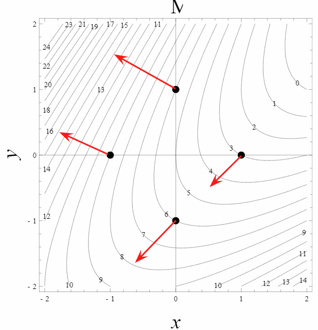
The figure shows a contour plot of a scalar field, \(\mu(x,y)\). Assume that \(x\) and \(y\) are measured in meters and that \(\mu\) is measured in kilograms. Four points are indicated on the plot.

-
Determine \(\frac{\partial\mu}{\partial x}\) and \(\frac{\partial\mu}{\partial
y}\) at each of the four points.
At each point, the partial derivative can be thought of as a ratio of the change in \(\mu\) when there is a small change in either \(x\) or \(y\) where the other variable is held constant (i.e., along either a horizontal or vertical line). To estimate a small change, we will use the smallest change available on the contour map: the change from the value at each indicated point to the nearest contour on both sides. This provides a slightly better estimate of the derivative than choosing only one side or the other, since the function may be changing more or less quickly in the positive or negative directions from the point. In cases where this is not possible due to the shapes of the contours, only the nearest side is used.
Top: \begin{align} \frac{\partial \mu}{\partial x}&=\frac{\mu_+ - \mu_-}{x_+ - x_-} \approx\frac{5 - 7}{0.25 + 0.2}= -4.4 kg/m\\ \frac{\partial \mu}{\partial y}&=\frac{\mu_+ - \mu_-}{y_+ - y_-} \approx\frac{7 - 5}{1.4 - 0.2}= 0.8 kg/m \end{align}
Left: \begin{align} \frac{\partial \mu}{\partial x}&=\frac{\mu_+ - \mu_-}{x_+ - x_-} \approx\frac{8 - 10}{-0.8 + 1.2}= -5 kg/m \\ \frac{\partial \mu}{\partial y}&=\frac{\mu_+ - \mu_-}{y_+ - y_-} \approx\frac{10 - 8}{0.4 + 1.1}= 1.3 kg/m \end{align}
Bottom: \begin{align} \frac{\partial \mu}{\partial x}&=\frac{\mu_+ - \mu_-}{x_+ - x_-}=\frac{6 - 7}{0 + 0.6}= -1.7 kg/m \\ \frac{\partial \mu}{\partial y}&=\frac{\mu_+ - \mu_-}{y_+ - y_-}=\frac{5 - 7}{0 + 1.4}= -1.4 kg/m \end{align}
Right: \begin{align} \frac{\partial \mu}{\partial x}&=\frac{\mu_+ - \mu_-}{x_+ - x_-} \approx\frac{3 - 4}{1 - 0.4}= -1.7 kg/m \\ \frac{\partial \mu}{\partial y}&=\frac{\mu_+ - \mu_-}{y_+ - y_-} \approx\frac{3 -4}{0 + 0.4}= -2.5 kg/m \end{align}
On a printout of the figure, draw a qualitatively accurate vector at each point corresponding to the gradient of \(\mu(x,y)\) using your answers to part a above. (How did you choose a scale for your vectors?)
Describe how the direction of the gradient vector is related to the contours on the plot and what property of the contour map is related to the magnitude of the gradient vector.
Here is an example of what your graph could look like, pay particular attention to the fact that the gradient points uphill and is perpindicular to the contour lines (lines of contant mu). Also gradient vectors near larger densities of contour lines should be larger in magnitude since the contour lines being close correspond to steeper increases.
-
Evaluate the gradient of
\(h(x,y)=(x+1)^2\left(\frac{x}{2}-\frac{y}{3}\right)^3\)
at the
point \((x,y)=(3,-2)\).
\begin{align} \vec{\nabla}h(x,y)\Bigg\vert_{(3,-2)} &= 2(x+1)\left(\frac{x}{2}-\frac{y}{3}\right)^3\, \hat{x} +3(x+1)^2\left(\frac{x}{2}-\frac{y}{3}\right)^2 \left(\frac{\hat{x}}{2}-\frac{\hat{y}}{3}\right)\Bigg\vert_{(3,-2)}\\ &=8\left(\frac{13}{6}\right)^3\, \hat{x} +48\left(\frac{13}{6}\right)^2 \left(\frac{\hat{x}}{2}-\frac{\hat{y}}{3}\right)\\ &=56 \left(\frac{13}{6}\right)^2\hat{x}-\frac{48}{3}\left(\frac{13}{6}\right)^2\hat{y}\approx 194 \hat{x}-75\hat{y} \end{align}
-
Determine \(\frac{\partial\mu}{\partial x}\) and \(\frac{\partial\mu}{\partial
y}\) at each of the four points.
- Gradient Practice
Find the gradient of each of the following functions:
-
\begin{equation}
f(x,y,z)=e^{(x+y)}+x^2 y^3 \ln \frac{x}{z}
\end{equation}
\begin{align} \vec{\nabla}f &= \frac{\partial f}{\partial x}\, \hat{x} +\frac{\partial f}{\partial y}\, \hat{y} +\frac{\partial f}{\partial z}\, \hat{z}\\ &= (e^{x+y} + 2xy^3\ln\frac{x}{z} + x^2y^3\frac{1}{x/z}\, \frac{1}{z})\hat{x}\\ &\qquad+ (e^{x+y}+3x^2y^2\ln\frac{x}{z})\hat{y}\\ &\qquad + x^2y^3\frac{1}{x/z}(-x/z^2)\hat{z}\\ &= (e^{x+y} + 2xy^3\ln\frac{x}{z} + xy^3)\hat{x} + (e^{x+y}+3x^2y^2\ln\frac{x}{z})\hat{y} - \frac{x^2y^3}{z}\hat{z} \end{align}
-
\begin{equation}
\sigma(\theta,\phi)=\cos\theta \sin^2\phi
\end{equation}
\begin{align} \vec{\nabla}\sigma &=\frac{\partial \sigma}{\partial r}\, \hat{r} +\frac{1}{r}\frac{\partial \sigma}{\partial \theta}\, \hat{\theta} +\frac{1}{r\sin\theta}\frac{\partial \sigma}{\partial \phi}\, \hat{\phi}\\ &= -\frac{\sin\theta\sin^2\phi}{r}\, \hat{\theta} + \frac{2\cos\theta\sin\phi\cos\phi}{r\sin\theta}\, \hat{\phi} \end{align}
-
\begin{equation}
\rho(s,\phi,z)=(s+3z)^2\cos\phi
\end{equation}
\begin{align} \vec{\nabla}\rho &= \frac{\partial \rho}{\partial s}\, \hat{s} +\frac{1}{s}\frac{\partial \rho}{\partial \phi}\, \hat{\phi} +\frac{\partial \rho}{\partial z}\, \hat{z}\\ &= 2(s+3z)\cos\phi\, \hat{s} - \frac{(s+3z)^2\sin\phi}{s}\, \hat{\phi} + 6(s+3z)\cos\phi\, \hat{z} \end{align}
-
\begin{equation}
f(x,y,z)=e^{(x+y)}+x^2 y^3 \ln \frac{x}{z}
\end{equation}
- Gauss's Law on a Cylindrical Shell
(6, 2, 2 pts)
Consider an infinite positively charged (dielectric) cylindrical shell of inner radius \(a\) and outer radius \(b\) with a cylindrically symmetric internal charge density \(\rho(\vec r)=\alpha\, e^{(ks)^2}\).
Answer each of the following questions:
- Use Gauss's Law and symmetry arguments to find the electric field at
each of the three radii below:
- \(s>b\)
- \(a<s<b\)
- \(s<a\)
- What dimensions do \(\alpha\) and \(k\) have?
- For \(\alpha=1\), \(k=1\), sketch the magnitude of the electric field as a function of \(s\).
-
By symmetry, the electric field only has a (cylindrical) radial component, and can only depend on the cylindrical radial coordinate \(s\), so \(\boldsymbol{\vec{E}}=E_s(s)\,\boldsymbol{\hat{s}}\).
Choose the Gaussian surface to be a finite cylinder of height \(L\)
and radius \(s\). Then the flux of \(\boldsymbol{\vec{E}}\) out of the cylinder is
\[\int_C\boldsymbol{\vec{E}}\cdot d\boldsymbol{\vec{A}}
= \int_C E_s(s)\,dA = 2\pi sLE_s\]
The charge \(Q_{enc}\) in the region \(R\) inside the cylinder \(C\) is
\[Q_{enc}=\int_R \rho\,d\tau\]
so Gauss's Law tells us that
\[E_s = \frac{Q_{enc}}{2\pi sL\epsilon_0}\]
- For \(s>b\), the enclosed charge is \[Q_{enc}=\int_0^{2\pi}\int_0^L\int_a^b \rho s\,ds\,dz\,d\phi = 2\pi L \int_a^b \alpha\,e^{(ks)^2}\,s\,ds = \frac{\pi L\alpha}{k^2} e^{(ks)^2}\bigg|_a^b\] so that \[E_s = \frac{\alpha}{2sk^2\epsilon_0}\left(e^{(kb)^2}-e^{(ka)^2}\right)\]
- For \(a<s<b\), the only thing that changes is the limits, and the enclosed charge is \[Q_{enc} = \frac{\pi L\alpha}{k^2} e^{(ks)^2}\bigg|_a^s\] so that \[E_s = \frac{\alpha}{2sk^2\epsilon_0}\left(e^{(ks)^2}-e^{(ka)^2}\right)\]
- For \(s<a\), \(Q_{enc}=0\), so \(E_s=0\).
- The quantity \(ks\) is dimensionless, and \(s\) has the dimensions of length, so \(k\) must have the dimensions of inverse length. Similarly, since \(\rho\) is a (volume) charge density, it has dimensions of \(\frac{\mathrm{charge}}{\mathrm{length}^3}\). Since the exponential factor must be dimensionless, these are also the dimensions of \(\alpha\).
Also setting \(a=1\), \(b=2\), and \(\epsilon_0=1\) yields a graph of the form below.

- Use Gauss's Law and symmetry arguments to find the electric field at
each of the three radii below:
- Flux Through a Cone
(6 pts)
Find the flux through a cone (with no cap!) of height \(H\) and radius \(R\) due to the vector field \(\vec{F} = C\,z\,\hat{z}\). The cone has its vertex at the origin, opens upward symmetrically around the z-axis. Orient your area elements so that upward pointing fields contribute positive flux.
This problem can be solved in either cylindrical and spherical coordinates.
Cylindrical Coordinates:
Chop the cone along slanted vertical lines \begin{align} \phi =\text{constant}&\Rightarrow d\phi=0\\ z=\frac{H}{R}\, s &\Rightarrow dz=\frac{H}{R}\, ds \end{align}
and horizontal circles \begin{align} s=\text{constant}&\Rightarrow ds=0\\ z=\text{constant}&\Rightarrow dz=0 \end{align}
Choose \(d\vec{r}_1\) and \(d\vec{r}_2\) so that the cross product gives an upward pointing vector. Find \(d\vec{A}=d\vec{r}_1\times d\vec{r}_2\). \begin{align} d\vec{r}_1 &= ds\, \hat{s}+\cancel{s\, d\phi\, \hat{\phi}}+dz\, \hat{z}\\ &= ds\,\left(\hat{s}+\frac{H}{R}\, \hat{z}\right)\\ d\vec{r}_2&=\cancel{ds\, \hat{s}}+s\, d\phi\, \hat{\phi}+\cancel{dz\, \hat{z}}\\ &= s\, d\phi\, \hat{\phi}\\ d\vec{A}&=d\vec{r}_1\times d\vec{r}_2\\ &= ds\,\left(\hat{s}+\frac{H}{R}\, \hat{z}\right)\times s\, d\phi\, \hat{\phi}\\ &= s\, ds\, d\phi\left(\hat{z}- \frac{H}{R}\, \hat{s} \right) \end{align} Putting all the pieces together, we have: \begin{align} \text{Flux}&=\int \vec{F}\cdot\vec{A}\\ &=\int_0^{2\pi} \int_0^R C\,z\,\hat{z}\cdot s\, ds\, d\phi\left(\hat{z}- \cancel{\frac{H}{R}\, \hat{s} }\right)\\ &=\int_0^{2\pi} \int_0^R C\,\frac{H}{R}\, s^2\, ds\, d\phi\\ &=2\pi C\,\frac{H}{R}\,\frac{1}{3} R^3\\ &=\frac{2\pi C}{3} HR^2 \end{align}
Spherical Coordinates:
Chop the cone along horizontal circles \begin{align} r=\text{constant}&\Rightarrow dr=0\\ \theta=\text{constant}&\Rightarrow d\theta=0 \end{align}
and along radial lines \begin{align} \phi=\text{constant}&\Rightarrow d\phi=0\\ \theta=\text{constant}&\Rightarrow d\theta=0 \end{align}
Choose \(d\vec{r}_1\) and \(d\vec{r}_2\) so that the cross product gives an upward pointing vector. Find \(d\vec{A}=d\vec{r}_1\times d\vec{r}_2\). \begin{align} d\vec{r}_1&=dr\, \hat{r}+\cancel{r\, d\theta\, \hat{\theta}} +\cancel{r\sin\theta\, d\phi\, \hat{\phi}}\\ &=dr\, \hat{r}\\ d\vec{r}_2&=\cancel{dr\, \hat{r}}+\cancel{r\, d\theta\, \hat{\theta}} +r\sin\theta\, d\phi\, \hat{\phi}\\ &=r\sin\theta\, d\phi\, \hat{\phi}\\ d\vec{A}&=d\vec{r}_1\times d\vec{r}_2\\ &=dr\, \hat{r}\times r\sin\theta\, d\phi\, \hat{\phi}\\ &=-r\sin\theta\, dr\, d\phi\, \hat{\theta} \end{align}
When we take the dot product of the vector field with the unit normal to the cone, we will have to evaluate \(-\hat{z}\cdot\hat{\theta}=\sin{\theta}\) which you can see most easily by drawing a picture. Also recall that \(z=r\cos\theta\). Putting all the pieces together, we have: \begin{align} \text{Flux}&=\int \vec{F}\cdot\vec{A}\\ &= -\int_0^{2\pi} \int_0^{\sqrt{H^2+R^2}} C\,z\,\hat{z}\cdot r\sin\theta\, dr\, d\phi\, \hat{\theta}\\ &= \int_0^{2\pi} \int_0^{\sqrt{H^2+R^2}} C\,r^2\cos\theta\, \sin^2\theta\, dr\, d\phi\\ &= 2\pi C\,\left.\frac{r^3}{3}\right\vert_0^{\sqrt{H^2+R^2}} \frac{H}{\sqrt{H^2+R^2}}\left(\frac{R}{\sqrt{H^2+R^2}}\right)^2\\ &= \frac{2\pi C}{3} HR^2 \end{align}