Contemporary Challenges: Fall-2024
Homework 5 (SOLUTION): Due 23 Friday 11/15
- Flute and boundary conditions
S1 5088S
Adapted from Q2M.1 from Chpt 2 of Unit Q, 3rd Edition
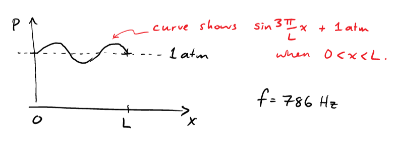
Waves of pressure (sound waves) can travel through air. When there are boundary conditions on a sound wave, the allowed frequencies become discretized (i.e. there is a discrete set of possible values). The same thing happens in quantum mechanics with "matter waves". Before getting fully into quantum mechanics, I want to warm up with musical examples. The PDE for pressure waves in a column of air is \begin{align} \frac{\partial^2p}{\partial t^2}=v_\text{s}^2\frac{\partial^2p}{\partial x^2} \end{align} where \(p\) is the pressure at time \(t\) and position \(x\), and \(v_\text{s}\) is a constant called the the speed of sound in air. We will look for solutions of the form \(p(x,t) = \sin(kx)\cos(wt) + \text{constant}\). The pressure at the open end of a pipe is fixed at 1 atmosphere (this boundary condition is called a node, because pressure doesn't fluctuate). If a pipe has a closed end (which may or may not be true for a flute) the pressure at the closed end can fluctuate up and down (this boundary condition would be called an anti-node).
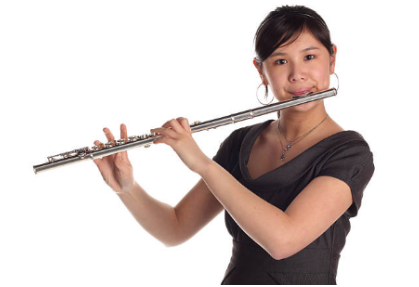
- A concert flute, shown above, is about 2 ft long. Its lowest pitch is middle C (about 262 Hz). On the basis of this evidence, should we consider a flute to be a pipe that is open at both ends, or at just one end? Support your argument with a quantitative comparison. (The end of the flute farthest from the mouth piece is clearly open. The other end of the flute seems to be closed, so if you claim that the flute is open at both ends, you should try to explain where the other open end is.)
If the flute has two open ends, there will be a pressure node at each end. Thus, the smallest value of \(k\) would be \(\pi/L\). This would give a standing wave \(P=P_0 \sin k x \sin k v t + (1\text{ atm})\) that will satisfy the PDE and the boundary conditions.
This curve would oscillate at an angular frequency \(\omega = v \pi/L\). The cycles per second frequency is \begin{align} f &= \frac{\omega}{ 2\pi} \\ &= \frac{v \pi}{2 \pi L}\\ &= \frac{v}{2 L} \\ &= \frac{340 \text{ m/s}}{2(0.6\text{ m})} = 262 \text{ Hz} \end{align}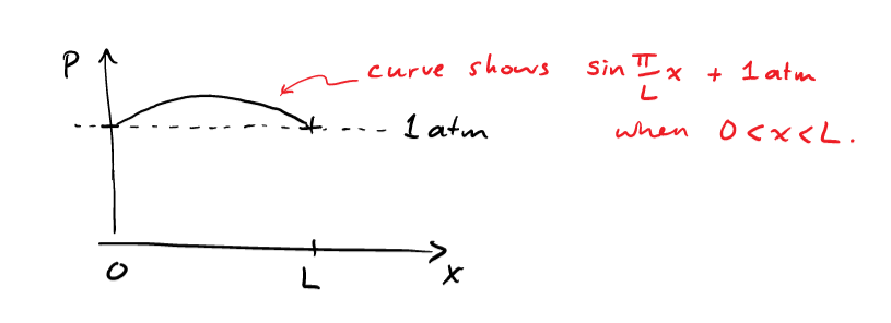
If the flute had one open end and one closed end, we expect a pressure node at one end and anti-node at the other end. The smallest value of \(k\) would be \((\pi/2)/L\).
This would give an angular frequency of \(\omega = v \pi /(2 L)\) and the cycles per second freqency is \begin{align} f &= \frac{\omega}{ 2\pi} \\ &= \frac{v \pi}{4 \pi L}\\ &= \frac{v}{4 L} \\ &= \frac{340 \text{ m/s}}{4(0.6\text{ m})} = 131 \text{ Hz} \end{align} I conclude that we should model the flute as open at both ends. The mouth piece has an open hole, and the "foot" of the flute has an open hole. Interestingly, a trumpet has a pressure anti-node at the mouth piece... so the boundary conditions for a trumpet are different than a flute.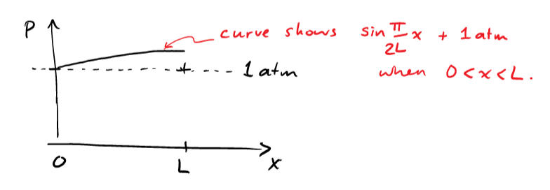
- What are the lowest three frequencies that can be played on a flute when all the finger holes are closed? Give you answer in units of Hz. Draw these frequencies on a spectrogram (vertical axis represents frequency, horizontal axis is time). Multiple horizonal lines at the same time represent the superposition of multiple frequencies.
Some other standing waves that satify the PDE and boundary conditions for a flute that is 0.6 m in length are
So, the lowest three frequencies are 262 Hz, 524 Hz, and 786 Hz.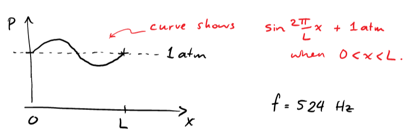
- Not graded this year - think about this question if you are interested: The orchestra is warming up their instruments. The air in the flute starts at 290 K and increases temperature to 300 K. How seriously does this affect the pitch of the flute? For reference, each step on a chromatic musical scale has a frequency 1.06 times higher than the one below it (1.06 = \(2^{1/12}\)). The conductor of the orchestra will be upset if the flute shifts from its correct frequency by \(\pm 1\%\). The speed of sound in a gas is \(v_s= \sqrt{(\gamma P_0/\rho_0)}\) where \(\gamma\) is a dimensionless constant, \(P_0\) is the ambient pressure and \(\rho_0\) is the gas's density. As the gas warms up, the density of air inside the flute drops (the equilibrium air pressure inside the flute does not change).
At 290 K we have \(v = 340\) m/s. The temperature rises to 300 K (\(3.4\%\) increase). We know \(v = \sqrt{\gamma P_0/\rho_0}\) where \(\gamma\) is a dimensionless number. When the flute warms up, \(P_0\) does not change (\(P_0 = 1\) atm). When the flute warms up, the density of air, \(\rho_0\), will change. Air behaves like an ideal gas, therefore \begin{align} P_0 V = N k_\text{B} T \rightarrow \frac{N}{V} = \frac{P_0}{k_\text{B} T} \end{align} The mass of air per unit volume is \begin{align} \rho_0 = \frac{m N}{V} = \frac{m P_0}{k_\text{B}T} \quad \text{ where \(m\) is average mass of an air molecule} \end{align} We can can substitute that into the velocity equation \begin{align} v = \sqrt{\frac{\gamma P_0 k_\text{B} T}{m P_0}} = \sqrt{\frac{\gamma k_\text{B} T}{m}} \end{align} When \(T\) increases by \(3.4\%\), \(v\) will increase by \(\frac{1}{2}3.4\% = 1.7\%\). We can see this by finding the ratio of \(v_1\) and \(v_2\). \begin{align} \frac{v_2}{v_1} = \frac{\sqrt{\frac{\gamma k_\text{B} T_2}{m}}}{\sqrt{\frac{\gamma k_\text{B} T_1}{m}}} = \sqrt{\frac{T_2}{T_1}} = \sqrt{\frac{300}{290}} = 1.017 \end{align} The pitch of the flute will be \(\omega = k v\) or \(f = k v /(2 \pi)\). The allowed wavenumbers, \(k\), will be the same. Therefore the pitch of the flute increases by \(1.7\%\). This is more than \(1/6\) of a chromatic step. The flute player will have to adjust the length of their flute.
- A concert flute, shown above, is about 2 ft long. Its lowest pitch is middle C (about 262 Hz). On the basis of this evidence, should we consider a flute to be a pipe that is open at both ends, or at just one end? Support your argument with a quantitative comparison. (The end of the flute farthest from the mouth piece is clearly open. The other end of the flute seems to be closed, so if you claim that the flute is open at both ends, you should try to explain where the other open end is.)
- Hot hydrogen atom
S1 5088S
Find the wavelength of the photon emitted during a \(n= 5\rightarrow4\) transition in a hydrogen atom.
Note: The energy levels in a hydrogen atom are \begin{align} E_n = \frac{-13.6 \text{ eV}}{n^2} \end{align} where \(n = 1,\ 2,\ 3,\ ...\)Calculate \(E_4\) and \(E_5\) \begin{align} E_4 = \frac{-13.6\text{ eV}}{4^2} = -0.85\text{ eV}\\ E_5 = \frac{-13.6\text{ eV}}{5^2} = -0.544\text{ eV}\\ \Delta E = 0.306 eV\\ \end{align} To find the wavelength in nanometers, I'll use the \(hc=1240\text{ eV.nm}\): \begin{align} \lambda = \frac{1240\text{ eV.nm}}{0.306\text{ eV}} = 4050\text{ nm} \end{align}
- Wavelength from a charge on a spring
S1 5088S
Suppose a charged particle is held in position by an electrostatic spring (i.e. the restoring force on the charge follows Hooke's law, \(F= -kx\)). The mass of the charge, and the spring constant, are such that the system has a natural frequency \(\omega = 10^{16}\text{ rad/s}\) (\(\omega\) is a fixed parameter in this question, not a variable). Find the wavelength of the photon emitted during a \(n= 1 \rightarrow 0\) transition.
By solving the Schrodinger equation for this situation, we know that the energy of the charged particle (i.e. the sum of the particle's kinetic energy, plus any potential energy stored in the spring) is given by \begin{align} E_n = \hbar \omega (n + \frac{1}{2}) \end{align} where \(n= 0,\ 1,\ 2,\ ...\)
Note: Due to the shape/symmetry of the wavefunctions for particles trapped by a springlike force, optical transitions only occur when \(\Delta n = \pm 1 \).
Sense making: Try approaching this question from a classical physics perspective. What wavelength of light would we expect from a charge that oscillates at \(\omega = 10^{16} \text{ rad/s}\)?\begin{align} &E_1 = \hbar \omega \left(\frac{3}{2}\right)\\ &E_0 = \hbar \omega \left(\frac{1}{2}\right)\\ &\Delta E = \hbar \omega = (1.05\times10^{-34})(10^{16})\text{ J}\\ & \quad \quad \quad \quad = 1.05\times 10^{-18} \text{ J} \\ & \quad \quad \quad \quad = 6.6 \text{ eV} \\ & \lambda = \frac{h c}{E_{photon}} = \frac{h c}{\hbar \omega} = \frac{1240 \text{ nm eV}}{6.6 \text{ eV}} = 190 \text{ nm} \end{align} If we applied a classical analysis (no quantum mechanics), we would expect light with frequency \(\omega/2\pi\). \begin{align} \lambda = \frac{c}{f} = \frac{hc}{hf} = \frac{hc}{\hbar \omega} = 190\text{ nm} \end{align} Exactly the same result.
- Light from an electron in a box
S1 5088S
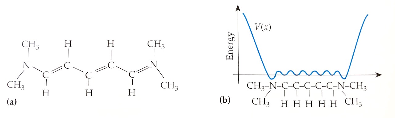
Suppose an electron is trapped in a box whose length is \(L= 1.2 \text{ nm}\). This is a coarse-grained model for an electron in a small molecule like cyanine (see Example Q11.1 in the textbook, and the figure above). If we solve the Schrodinger equation for this coarse-grained model, the possible energy levels for this electron are \begin{align} E = \frac{h^2 n^2}{8 m L^2} \end{align} where \(m\) is the mass of the electron and \(n= 1,\ 2,\ 3,\ ...\)
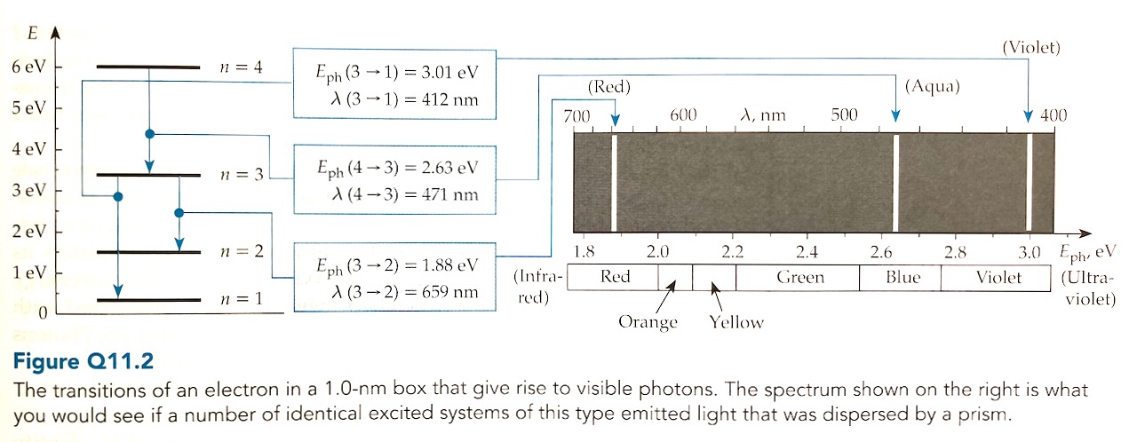
Draw a spectrum chart (like the righthand side of Figure Q11.2) illustrating all visible spectral lines (i.e. any wavelengths between infrared and ultraviolet) that can be emitted by a test tube full of cyanine molecules when every possible electronic transition is happening.
Note: Due to the shape/symmetries of electron wavefunctions in a box, optical transitions between energy levels only happen when \(\Delta n = n_\text{initial}-n_\text{final}\), is an odd integer.
Visible photons
The energy levels fro the electron are \begin{align} E_n &= \frac{h^2 n^2}{8 m L^2} \qquad \qquad \text{ where } L = 1.12\text{ nm}\\ &= \left[\frac{(6.6\times10^{-34})^2}{8 (9\times10^{-31}) (1.2\times10^{-9})^2}\right] n^2\\ &\approx [0.4\times10^{-19}\text{ J}]n^2\\ &=[0.25\text{ eV}]n^2 \end{align} First I'll look at transitions with \(\Delta n = 1\), for example \(n=4\) to \(n=3\). Now I'll check transitions with \(\Delta n=3\), for example \(n=4\) to \(n=1\).
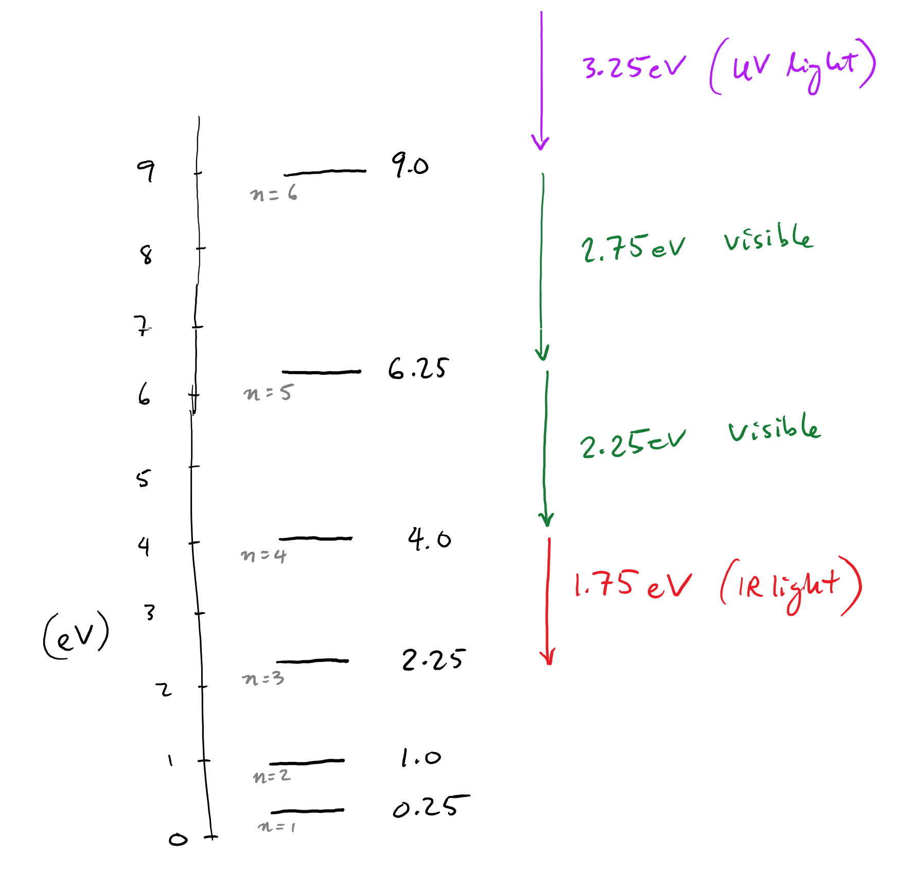 If \(\Delta n=5\) the system would emit photons of 3.75 eV or greater (outside the visible spectrum).
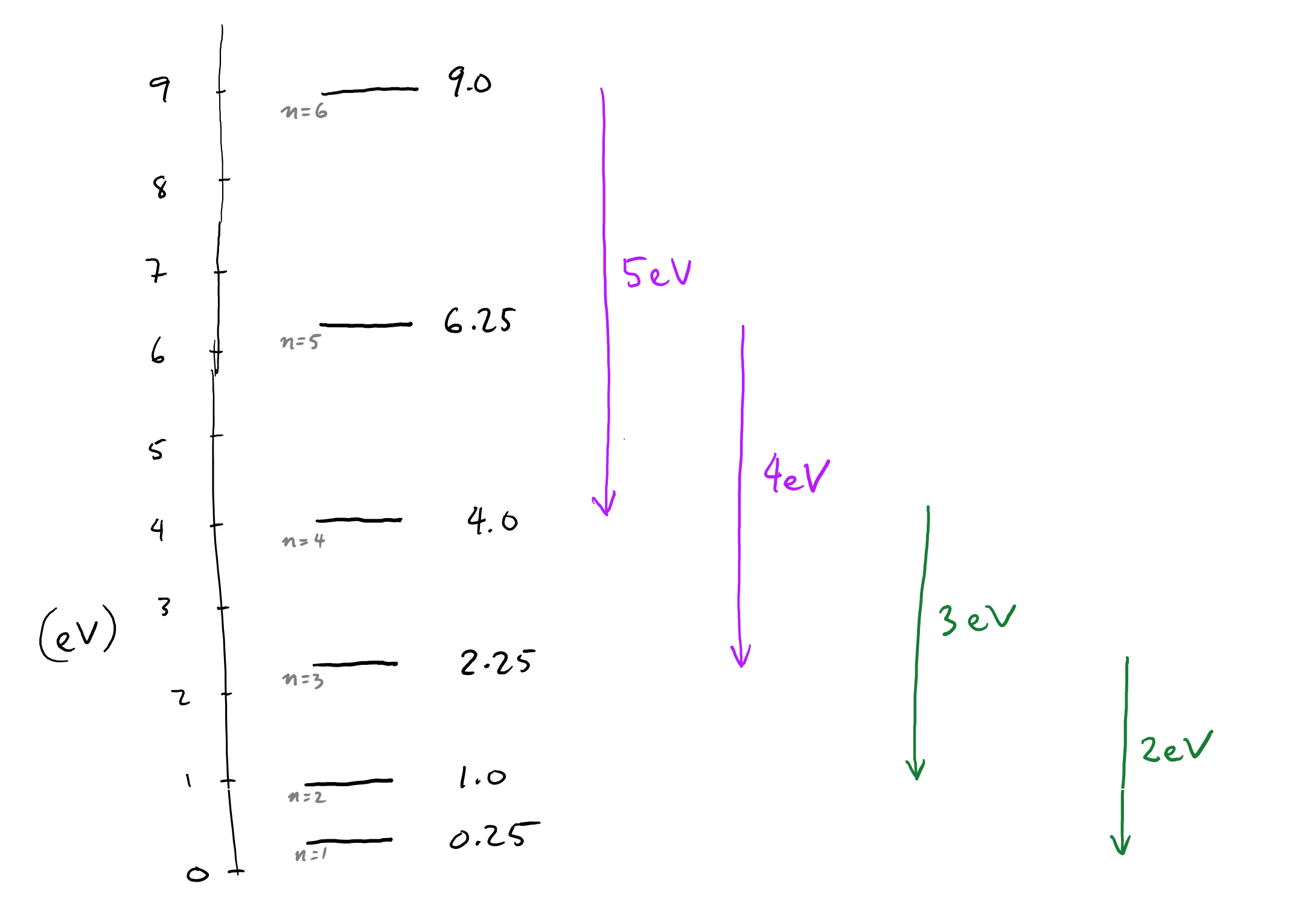
In conclusion, there are four energies of visible photons that this system could emit: 2 eV, 2.25 eV, 2.75 eV and 3 eV.