Contemporary Challenges: Fall-2024
Homework 4 (SOLUTION): Due 17 Friday 11/1

1. Helium heat capacity S1 5086S

   In class, we assumed that all monatomic gases have 3 degrees of freedom (\(f = 3\)). In this question, we explore the possibility that a monatomic gas might have additional degrees of freedom due to the electrons orbiting the nucleus. To answer this question, you will need to use the equipartition theorem and understand how quantized energy levels affect the application of the equipartition theorem.

   Helium is a monatomic gas at room temperature. An atom of helium can store energy by bumping its electron from its lowest orbital energy level to a higher orbital energy level. In particular, moving an electron from the lowest state to the first excited state would store an energy of 24.6 eV (24.6 electron-volts). Give a quantitative explanation (i.e. by comparing quantities) that shows we can ignore this energy storage mode when calculating the heat capacity of helium gas at ordinary temperatures.

   At \(T=293\) K, \(k_\text{B}T \approx 0.025\) eV. Thus, a system that accepts an energy quanta 24.6 eV is very unlikely to get that energy from the surrounding environment when \(T=293\) K, because that is 1000 times higher than \(k_BT\).

2. Heat Pump S1 5086S

   

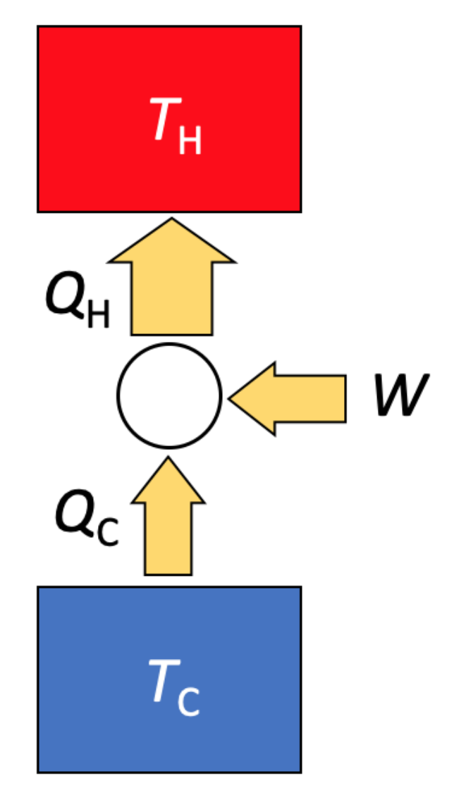
   The diagram shows a machine (the white circle) that moves energy from a cold reservoir to a hot reservoir. We will consider whether a machine like this is useful for heating a family home in the winter when the temperature inside the family home is \(T_\text{H}\), and the temperature outside the house is \(T_\text{C}\). To quantify the performance of this machine, I'm interested inthe ratio \(Q_\text{H}/W\), where \(Q_{\text{H}}\) is the heat energy entering the house, and \(W\) is the net energy input in the form of work. (\(W\) is the energy I need to buy from the electricity company to run an electric motor). Starting from the 1\(^{\text{st}}\) and 2\(^\text{nd}\) laws of thermodynamics, find the maximum possible value of \(Q_\text{H}/W\). This maximum value of \(Q_\text{H}/W\) will depend solely on the ratio of temperatures \(T_\text{H}\) and \(T_\text{C}\).

   We are tring to maximize the heat flowing into the high temperature reservoir for a given amount of work input. By the first law of thermodynamics we know that

   \[Q_{\text{C}}+W = Q_{\text{H}}\]

   If I fix W, then increasing \(Q_{\text{C}}\) will increase \(Q_\text{H}\).

   By the second law of thermodynamics we know \begin{align} -\frac{Q_{\text{C}}}{T_{\text{C}}} + \frac{Q_{\text{H}}}{T_{\text{H}}} \geq 0 \end{align}

   If we use the beggest \(Q_{\text{C}}\) then \begin{align} \frac{Q_{\text{C}}}{T_{\text{C}}} = \frac{Q_{\text{H}}}{T_{\text{H}}}\\ \rightarrow \frac{Q_{\text{C}}}{Q_{\text{H}}} = \frac{T_{\text{C}}}{T_{\text{H}}} \end{align}

   We can combine the two equations to get the efficiency: \begin{align*} \epsilon = \frac{Q_\text{H}}{W} &= \frac{Q_\text{H}}{Q_\text{H}-Q_\text{C}}\\[6pt] \frac{1}{\epsilon} &= \frac{Q_\text{H}-Q_\text{C}}{Q_\text{H}} \\[6pt] &= 1- \frac{Q_\text{C}}{Q_\text{H}} \\[6pt] &= 1- \frac{T_\text{C}}{T_\text{H}} \\[6pt] &= \frac{T_{\text{H}}-T_{\text{C}}}{T_\text{H}} \\[6pt] \epsilon &= \frac{T_\text{H}}{T_{\text{H}}-T_{\text{C}}} \end{align*}

   To understand this answer, I can consider a few special cases. If \(T_\text{H} = T_{\text{C}}\), then no work is needed. If \(T_{\text{C}}\rightarrow 0\), then \(Q_\text{H} = W\). All the heat must come from work.

   I'm also noticing that the difference in temperature between the reservoirs is going to be smaller than the temperature of the hot reservoirs, so I'm expecting efficiencies that are bigger than 1.

   Sensemaking: Choose realistic values of \(T_\text{H}\) and \(T_\text{C}\) to describe a family home on a snowy day. Based on your temperature estimates, what is the maximum possible value of \(Q_\text{H}/W\)?

   For a snowy day, let \(T_{\text{C}} = 270\) K and \(T_\text{H} = 290\) K.

   Substituting that into my equation, I get \(Q_\text{H}/W = 290/20 \approx 15\).

   That sounds great! How well do real heat pumps perform? See wikipedia: “Heat Pump”, subsection “performance considerations.” It says that \(Q_\text{H}/W \approx 3.2-4.5\) for a unit you can install at your house.

3. Photons Absorbed and Reradiated by Earth Estimation S1 5086S

   The energy of a single photon (a particle of light) is related to its wavelength:

   \[E_{\text{photon}} = \frac{hc}{\lambda}\]

   where \(h\) is Planck's constant, \(c\) is the speed of light, and \(\lambda\) is the wavelength of light.

   We've previously talked about how the Earth can function perfectly fine when all the energy we receive from the sun as photons centered in the visible spectrum is reradiated by the Earth as photons centered in the infrared spectrum.

   Use a coarse-grained model that:

   • all the energy we receive from the Sun is carried by yellow-green photons (\(\lambda = 560 \text{ nanometers}\) - the peak of the suns electromagnetic spectrum) and that
   • all this energy is re-radiated by Earth as infrared photons (\(\lambda = 10. \text{ micrometers}\), the peak of the electromagnetic spectrum)
   to estimate the ratio of the number of photons emitted by Earth to the number of photon incident on the Earth.

   In a situation where all the energy incident on the Earth is reradiated, the ratio of energy radiated by the Earth and energy from the Sun is 1:

   \begin{align*} \frac{E_{\text{Earth}}}{E_{\text{Sun}}} = 1 \end{align*}

   These energies can be expressed as the product of the number of photons and the energy for each photon.

   \begin{align*} \frac{E_{\text{Earth}}}{E_{\text{Sun}}} &= \frac{N_{\text {infrared}}E_{\text{infrared}}}{N_{\text{green}}E_{\text{green}}} \\ &= 1 \end{align*}

   Rearranging, I can relate the number of photons to the energies of the photons, and then the energies of the photons to the wavelengths of the photons:

   \begin{align*} \frac{N_{\text {infrared}}}{N_{\text{green}}} &= \frac{E_{\text{green}}}{E_{\text{infrared}}} \\ &= \frac{\frac{hc}{\lambda_{\text{green}}}}{\frac{hc}{\lambda_{\text{infrared}}}} \\ &= \frac{{\lambda_{\text{infrared}}}}{{\lambda_{\text{green}}}}\\ &= \frac{10 \times 10^{-6} \text{ m}}{560 \times 10^{-9} \text{ m}}\\ &\approx 18 \end{align*}

   It looks like for every green photon from the sun incident on the Earth, there are about 18 infrared photons emitted from the Earth.

   (Of course, each object emits its own spectrum of photons, and this calculation makes simiplifying assumption that all the photons are at the peak of the spectrum.)

4. Standing Waves S1 5086S A standing wave is produced with two identical traveling waves move past each other traveling in opposite directions.

   • Convince yourself that a standing wave

     \[y_S(x,t) = 2\sin[(\pi \text{ m}^{-1}) x]\cos[(\pi \text{ s}^{-1}) t]\]

     is by a superposition of waves:

     \[y(x,t) = \sin[(\pi \text{ m}^{-1}) x \pm (\pi \text{ s}^{-1}) t]\]

     You can do this through the use of trig identities or by graphing the different functions and observing the shapes (turn in screen shots if you go this route).

     1. Trig Identities Looking up trig identities, I see that:

        \[\sin(\alpha + \beta) + \sin(\alpha - \beta) = 2\sin\alpha\cos\beta\]

        in this case, let \(\alpha = (\pi \text{ m}^{-1}) x\) and \(\beta = (\pi \text{ s}^{-1}) t\) :

        \begin{align*} \sin[(\pi \text{ m}^{-1}) x + (\pi \text{ s}^{-1}) t] + \sin[(\pi \text{ m}^{-1}) x - (\pi \text{ s}^{-1}) t] = 2\sin[(\pi \text{ m}^{-1}) x]\cos[(\pi \text{ s}^{-1}) t] \end{align*}

     2. Graphing

        You can play around with my Desmos graph.

   • Show that the standing wave equation solves the wave equation for a wave on a string.

     I'll do this by plugging the solution back into the original differential equation:

     \[\frac{\partial ^2 y}{\partial x^2} = \frac{\mu}{T} \frac{\partial ^2 y}{\partial t^2}\]

     First, let me do this with symbols. Let \(k= \pi \text{ m}^{-1})\) and \(\omega = (\pi \text{ s}^{-1})\) so that the solution is:

     \[y_S(x,t)= 2 \sin kx \cos \omega t\]

     First, I take all the partial derivatives:

     \begin{align*} \frac{\partial y_S}{\partial x} = 2k\cos kx\cos \omega t \\[6pt] \frac{\partial^2 y}{\partial x^2} = -2k^2\sin kx\cos \omega t \\[6pt] \frac{\partial y_S}{\partial t} = -2\omega \sin kx\sin \omega t \\[6pt] \frac{\partial y_S}{\partial t} = -2\omega^2\sin kx\cos \omega t \\[6pt] \end{align*}

     Plugging these into the wave equation:

     \begin{align*} \frac{\partial ^2 y}{\partial x^2} &= \frac{\mu}{T} \frac{\partial ^2 y}{\partial t^2} \\[6pt] \cancel{-2} k^2 \cancel{\sin kx\cos \omega t} &= \frac{\mu}{T} \Big( \cancel{-2} \omega^2 \cancel{\sin kx\cos \omega t} \Big) \\[6pt] \Big(\frac{k}{\omega}\Big)^2 = \frac{\mu}{T} \end{align*}

     So, \(y_S\) is a solution, as long as \(\Big(\frac{k}{\omega}\Big)^2 = \frac{\mu}{T}\). It turns out that both sides are equal to the inverse speed squared of the wave:

     \[ \frac{1}{v^2} = \Big(\frac{k}{\omega}\Big)^2 = \frac{\mu}{T}\]