Contemporary Challenges: Fall-2023
Homework 4 (SOLUTION): Due 17 Friday 11/3
- Helium heat capacity
S1 4743S
In class, we assumed that all monatomic gases have 3 degrees of freedom (\(f = 3\)). In this question, we explore the possibility that a monatomic gas might have additional degrees of freedom due to the electrons orbiting the nucleus, or the rotation of the nucleus. To answer this question, you will need to use the equipartition theorem and understand how quantized energy levels affect the application of the equipartition theorem.
(a) An atom of helium can store energy by bumping its electron from its lowest orbital energy level to a higher orbital energy level. Moving an electron from the lowest state to the first excited state would store an energy of 24.6 eV (24.6 electron-volts). Give a quantitative explanation (i.e. by comparing quantities) that shows we can ignore this energy storage mode when calculating the heat capacity of helium gas at ordinary temperatures.
(b) The helium-4 nucleus can be modelled as a solid spherical object with mass \(m\), radius \(r\), and moment of inertia \(I=(2/5)mr^2\). If the nucleus starts to rotate, it would have rotational kinetic energy \(K_{\text{rotation}}=L^2/(2I)\), where \(L\) is the angular momentum. Usually the helium-4 nucleus has \(L = 0\), however, it can be excited to a non-zero angular momentum state with \(L \approx \hbar\), or \(2\hbar\), or \(3\hbar\), etc. (\(L\) is quantized). Give a quantitative explanation that shows we can ignore this energy storage mode when calculating the heat capacity of helium gas at ordinary temperatures.
(a) At \(T=293\) K, \(k_\text{B}T \approx 0.025\) eV. Thus, a system that accepts an energy quanta 24.6 eV is very unlikely to get that energy from the surrounding environment when \(T=293\) K, because that is 1000 times higher than \(k_BT\).
(b) No solution has been written yet.
- Flute and boundary conditions
S1 4743S
Adapted from Q2M.1 from Chpt 2 of Unit Q, 3rd Edition
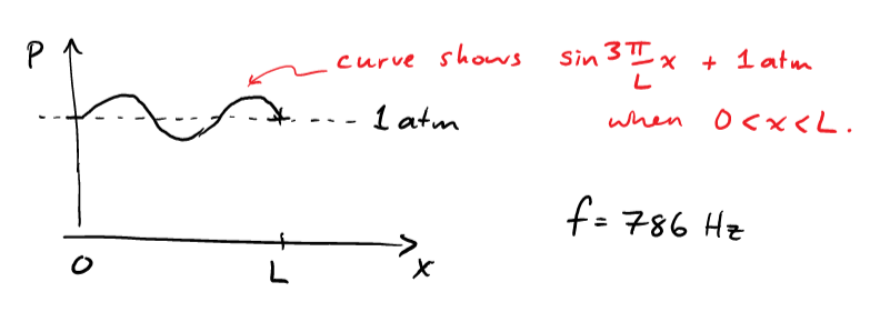
Waves of pressure (sound waves) can travel through air. When there are boundary conditions on a sound wave, the allowed frequencies become discretized (i.e. there is a discrete set of possible values). The same thing happens in quantum mechanics with "matter waves". Before getting fully into quantum mechanics, I want to warm up with musical examples. The PDE for pressure waves in a column of air is \begin{align} \frac{\partial^2p}{\partial t^2}=v_\text{s}^2\frac{\partial^2p}{\partial x^2} \end{align} where \(p\) is the pressure at time \(t\) and position \(x\), and \(v_\text{s}\) is a constant called the the speed of sound in air. We will look for solutions of the form \(p(x,t) = \sin(kx)\cos(wt) + \text{constant}\). The pressure at the open end of a pipe is fixed at 1 atmosphere (this boundary condition is called a node, because pressure doesn't fluctuate). If a pipe has a closed end (which may or may not be true for a flute) the pressure at the closed end can fluctuate up and down (this boundary condition would be called an anti-node).
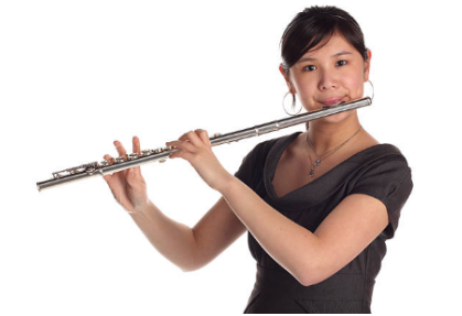
- A concert flute, shown above, is about 2 ft long. Its lowest pitch is middle C (about 262 Hz). On the basis of this evidence, should we consider a flute to be a pipe that is open at both ends, or at just one end? Support your argument with a quantitative comparison. (The end of the flute farthest from the mouth piece is clearly open. The other end of the flute seems to be closed, so if you claim that the flute is open at both ends, you should try to explain where the other open end is.)
If the flute has two open ends, there will be a pressure node at each end. Thus, the smallest value of \(k\) would be \(\pi/L\). This would give a standing wave \(P=P_0 \sin k x \sin k v t + (1\text{ atm})\) that will satisfy the PDE and the boundary conditions.
This curve would oscillate at an angular frequency \(\omega = v \pi/L\). The cycles per second frequency is \begin{align} f &= \frac{\omega}{ 2\pi} \\ &= \frac{v \pi}{2 \pi L}\\ &= \frac{v}{2 L} \\ &= \frac{340 \text{ m/s}}{2(0.6\text{ m})} = 262 \text{ Hz} \end{align}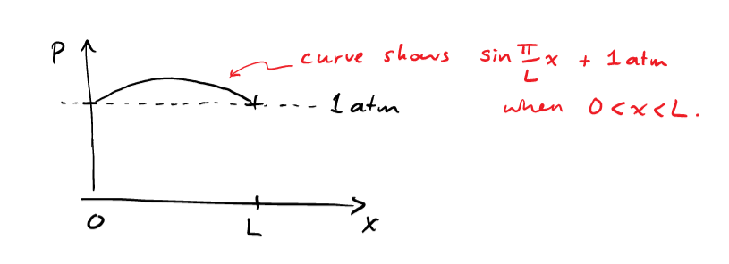
If the flute had one open end and one closed end, we expect a pressure node at one end and anti-node at the other end. The smallest value of \(k\) would be \((\pi/2)/L\).
This would give an angular frequency of \(\omega = v \pi /(2 L)\) and the cycles per second freqency is \begin{align} f &= \frac{\omega}{ 2\pi} \\ &= \frac{v \pi}{4 \pi L}\\ &= \frac{v}{4 L} \\ &= \frac{340 \text{ m/s}}{4(0.6\text{ m})} = 131 \text{ Hz} \end{align} I conclude that we should model the flute as open at both ends. The mouth piece has an open hole, and the "foot" of the flute has an open hole. Interestingly, a trumpet has a pressure anti-node at the mouth piece... so the boundary conditions for a trumpet are different than a flute.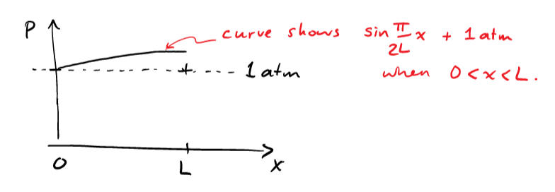
- What are the lowest three frequencies that can be played on a flute when all the finger holes are closed? Give you answer in units of Hz. Draw these frequencies on a spectrogram (vertical axis represents frequency, horizontal axis is time). Multiple horizonal lines at the same time represent the superposition of multiple frequencies.
Some other standing waves that satify the PDE and boundary conditions for a flute that is 0.6 m in length are
So, the lowest three frequencies are 262 Hz, 524 Hz, and 786 Hz.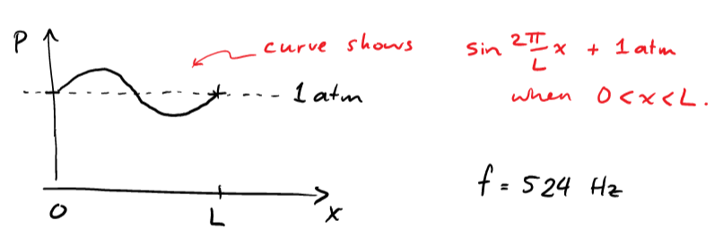
- Not graded this year - think about this question if you are interested: The orchestra is warming up their instruments. The air in the flute starts at 290 K and increases temperature to 300 K. How seriously does this affect the pitch of the flute? For reference, each step on a chromatic musical scale has a frequency 1.06 times higher than the one below it (1.06 = \(2^{1/12}\)). The conductor of the orchestra will be upset if the flute shifts from its correct frequency by \(\pm 1\%\). The speed of sound in a gas is \(v_s= \sqrt{(\gamma P_0/\rho_0)}\) where \(\gamma\) is a dimensionless constant, \(P_0\) is the ambient pressure and \(\rho_0\) is the gas's density. As the gas warms up, the density of air inside the flute drops (the equilibrium air pressure inside the flute does not change).
At 290 K we have \(v = 340\) m/s. The temperature rises to 300 K (\(3.4\%\) increase). We know \(v = \sqrt{\gamma P_0/\rho_0}\) where \(\gamma\) is a dimensionless number. When the flute warms up, \(P_0\) does not change (\(P_0 = 1\) atm). When the flute warms up, the density of air, \(\rho_0\), will change. Air behaves like an ideal gas, therefore \begin{align} P_0 V = N k_\text{B} T \rightarrow \frac{N}{V} = \frac{P_0}{k_\text{B} T} \end{align} The mass of air per unit volume is \begin{align} \rho_0 = \frac{m N}{V} = \frac{m P_0}{k_\text{B}T} \quad \text{ where \(m\) is average mass of an air molecule} \end{align} We can can substitute that into the velocity equation \begin{align} v = \sqrt{\frac{\gamma P_0 k_\text{B} T}{m P_0}} = \sqrt{\frac{\gamma k_\text{B} T}{m}} \end{align} When \(T\) increases by \(3.4\%\), \(v\) will increase by \(\frac{1}{2}3.4\% = 1.7\%\). We can see this by finding the ratio of \(v_1\) and \(v_2\). \begin{align} \frac{v_2}{v_1} = \frac{\sqrt{\frac{\gamma k_\text{B} T_2}{m}}}{\sqrt{\frac{\gamma k_\text{B} T_1}{m}}} = \sqrt{\frac{T_2}{T_1}} = \sqrt{\frac{300}{290}} = 1.017 \end{align} The pitch of the flute will be \(\omega = k v\) or \(f = k v /(2 \pi)\). The allowed wavenumbers, \(k\), will be the same. Therefore the pitch of the flute increases by \(1.7\%\). This is more than \(1/6\) of a chromatic step. The flute player will have to adjust the length of their flute.
- A concert flute, shown above, is about 2 ft long. Its lowest pitch is middle C (about 262 Hz). On the basis of this evidence, should we consider a flute to be a pipe that is open at both ends, or at just one end? Support your argument with a quantitative comparison. (The end of the flute farthest from the mouth piece is clearly open. The other end of the flute seems to be closed, so if you claim that the flute is open at both ends, you should try to explain where the other open end is.)
- Bugle
S1 4743S
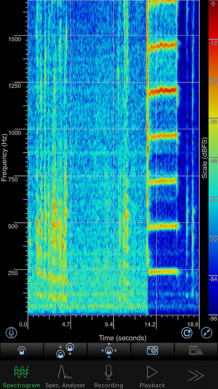
In this question, you will analyze a frequency spectrum recorded from a bugle (a demonstration might be done during class). We'll compare the real bugle data to a coarse-grain model, and consider what might be missing from the coarse-grain model.
I found two articles on the internet (links 1 & 2 below) that helped me understand the physics of standing waves in brass instruments.
A didgeridoo is an example of a “closed-open” pipe with a fixed inner diameter. The didgeridoo makes an ethereal/otherworldly sound. Trumpets, trombones and bugles are also “closed-open” pipes, but the inside diameter of the pipe grows bigger at the end of the instrument. To get the “classical” pattern of frequencies, the shape of this flare is critical (trumpets, trombones and bugles all have a similiar flare).
The spectrogram shown below was recorded when I played a note on the bugle. This note is a superposition of the bugle's 2nd resonance (240 Hz), the 4th resonance (480 Hz), the 6th resonance (720 Hz) and so forth. Other resonances were not excited when I played this note. (Other resonances could be excited if I played a different note). I am using a standard convention of numbering the lowest resonant frequency as #1, the next highest resonant frequency as #2, and so forth.
- Draw pressure-vs.-position graphs illustrating four of the allowed standing waves inside a pipe with closed-open boundary conditions. The x-axis represents the distance along the pipe. \(x = 0\) is the mouthpiece (the closed boundary) and \(x = L\) is the open end of the pipe. Draw 4 different graphs. The first graph corresponds to the first resonance. The second graph corresponds to the second resonance and so forth.
- Using your four graphs, find expressions for the wavelength and frequency of each standing wave. I'm looking for symbollic expressions in terms of \(L\) and the \(v_s\). Make sure that you can deduce the wavelength from your graphs, rather than resorting to a textbook formula.
- The fourth resonance of the actual bugle is 480 Hz. Find the length of straight pipe for which the coarse-grained model matches this experimental result. Use this estimated length to determine if the coarse-grained model correctly predicts resonant frequency #2 (numerical answer).
- Present your analysis by drawing side-by-side spectrograms. On the first spectrogram, show the resonant frequencies #2 and #4 predicted by the coarse grain model. On the second spectrogram, show the resonant frequencies #2 and #4 measured from the bugle. Speculate on what might cause the descrepancy between the model and the real world.
Some helpful figures from the internet articles:
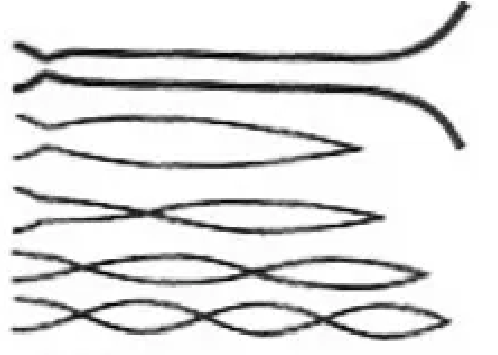
Figure 1: Approximate pressure distribution for the first four modes in a trumpet. Note that the “turning point” moves outward in the bell as the frequency increases. Mode frequencies are nearly in the ratios 0.8 : 2 : 3 : 4. 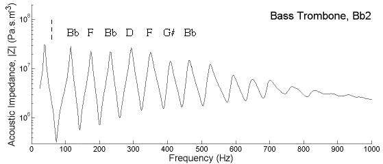
Figure 2: The resonant modes of a brass instrument can be determined by finding the peaks in the acoustic impendance. The graphs below show waves that have an anti-node a \(x=0\) and a node at \(x=L\). Outside bugle (\(x>L\)) the air pressure returns to normal. I have not shown the small ripple of sound leaving the bugle because pressure oscillations inside the bugle are much bigger than outside).
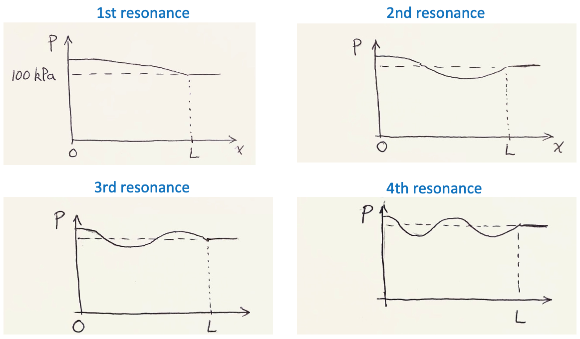
Examining the graphs above, the first resonance fits a quarter wavelength inside the bugle (\(\lambda _1/4 =L\)). The second resonance fits three "quarter wavelengths" inside the bugle. The third resonance fits five "quarter wavelengths" inside the bugle. The four resonance fits seven "quarter wavelengths" inside the bugle. Therefore, the wavelengths are \begin{align} \lambda _1 = 4L\\ \lambda _2 = 4L/3\\ \lambda _3 = 4L/5\\ \lambda _4 = 4L/7\\ \end{align} The corresponding frequencies (\(f=v / \lambda\)) are \begin{align} f_1=v/4L\\ f_2=3v/4L\\ f_3=5v/4L\\ f_4=7v/4L\\ \end{align}
- Using the straight-pipe model to get \(f_4=480\) Hz, the length of the pipe would be... \begin{align} f_4&=\frac{7v}{4L}\\ L&=\frac{7v}{4f_4}\\ &=\frac{7(340 \text{ m/s})}{4(480 \text{ s}^{-1})}\\ &=1.24 \text{ m} \end{align}
If we assume \(L = 1.24\) m, the numerical values for other resonant frequencies are \begin{align} f_1 = v/4L = 340 \text{ m/s}/(4\times1.24 \text{m}) = 69 \text{ Hz}\\ f_2 = 3v/4L = 206 \text{ Hz}\\ f_3 = 5v/4L = 343 \text{ Hz}\\ f_4 = 7v/4L = 480 \text{ Hz}\\ \end{align}
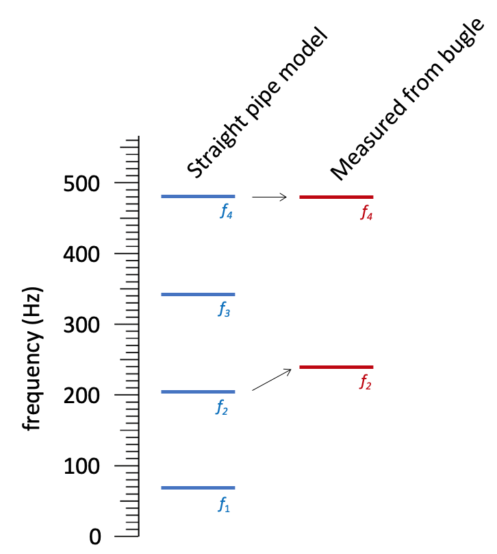
In summary, when we fit the model to the data using the \(f_4\) resonance, the \(f_2\) resonance does not fit. The measured \(f_2\) is higher than predicted by the straight-pipe model. How do I make sense of this? The information from Univ. of New South Wales says: "in the rapidly flaring bell, the long waves (with the low pitches) could be said to be 'least able to follow' the curve of the bell and so are effectively reflected earlier than are the shorter waves. (This is because their wavelengths are very much longer than the radius of curvature of the bell.) One might say therefore that the long waves 'see' an effectively shorter pipe."