Problem-Solving: Fall-2024
Tutorial 3 (Required) (SOLUTION): Due W3 D2

1. Sphere in Cylindrical Coordinates S1 5143S Find the surface area of a sphere using cylindrical coordinates. Note: The fact that you can describe spheres nicely in cylindrical coordinates underlies the equal area cylindrical map project that allows you to draw maps of the earth where everything has the correct area, even if the shapes seem distorted. If you want to plot something like population density, you need an area preserving map projection.

   Recall that in cylindrical coordinates we have \[d\boldsymbol{\vec r}=ds\,\boldsymbol{\hat s} +s\,d\phi\,\boldsymbol{\hat\phi}+dz\,\boldsymbol{\hat z}\] and that infinitesimal distance is given by \(d\ell=|d\boldsymbol{\vec r}|\). Chop up the surface of the sphere as usual along lines of latitude and longitude. Along a line of latitude, only \(\phi\) is changing, so \(ds=0=dz\) so \[d\ell_1=|s\,d\phi\,\boldsymbol{\hat\phi}|=s\,d\phi.\]

   Along a line of longitude, only \(\phi\) is constant; both \(s\) and \(z\) are changing. So we need to find a relationship between \(ds\) and \(dz\). The equation of a sphere of radius \(R\) in cylindrical coordinates is \(s^2+z^2=R^2\), where \(R\) is a constant. Zapping this equation with \(d\) yields \(2s\,ds+2z\,dz=0\). Now we can write \begin{align} d\ell_2&=\vert d\vec{r}\vert\\ &=|ds\,\boldsymbol{\hat s}+dz\,\boldsymbol{\hat z}|\\ &=\left|-\frac{z}{s}dz\,\boldsymbol{\hat s}+dz\,\boldsymbol{\hat z}\right|\\ &=\sqrt{\frac{z^2+s^2}{s^2}}dz\\ &=\frac{R}{s}dz \end{align} where it is important to remember that \(s\) is now a function of \(z\).

   The area element on the sphere is therefore the product of these two infinitesimal lengths, often written as \begin{align} dA &= (d\ell_1)(d\ell_2)\\ &=\vert d\vec{r}_1\times d\vec{r}_2\vert\\ &= (s\,d\phi)\left(\frac{R}{s}dz\right)\\ &=R\,d\phi\,dz. \end{align}

   It remains only to integrate this expression, obtaining \[A=\int_{-R}^R\int_0^{2\pi} R\,d\phi\,dz = 4\pi R^2.\] Setting up this integral may be a challenge, but the integration itself is even easier than in spherical coordinates!

2. Charge on a Spiral S1 5143S (8pts) A charged spiral in the \(x,y\)-plane has 6 turns from the origin out to a maximum radius \(R\) , with \(\phi\) increasing proportionally to the distance from the center of the spiral. Charge is distributed on the spiral so that the charge density increases linearly as the radial distance from the center increases. At the center of the spiral the linear charge density is \(0~\frac{\textrm{C}}{\textrm{m}}\). At the end of the spiral, the linear charge density is \(13~\frac{\textrm{C}}{\textrm{m}}\). What is the total charge on the spiral?

   Let's start by finding the charge density on the spiral. We know that the charge density increases linearly with the distance from the center of the spiral, so our linear charge density will be proportional to the radius, \(s\). (Notice the two different uses of the word “linear”!) We also know that at the max radius, \(R\), we will have a linear charge density of \(13~\frac{\textrm{C}}{\textrm{m}}\), so we can solve for the proportionality constant, which we'll call \(\alpha\) \begin{align} \lambda(s) &= \alpha s\\ 13 ~\frac{\textrm{C}}{\textrm{m}} &= \alpha R\\ \Rightarrow \alpha&=\frac{13~\frac{\textrm{C}}{\textrm{m}}}{R}\\ \lambda(s) &= \left(13~\frac{\textrm{C}}{\textrm{m}}\right) \frac{s}{R} \end{align}

   Looking at our spiral:
   

   

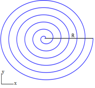
   We will chop up the spiral into little pieces and find the charge \(\lambda\, d\ell\) on each little piece. Then we will add up (integrate) the charge from each of the little pieces. (Sensemaking: Note that \(\lambda(s)\) has the correct units, since \(s/R\) is unitless---I will suppress the \(\frac{\textrm{C}}{\textrm{m}}\) and restore it at the very end.)

   So the next thing we need to find is \(d\ell\) on a little piece of the spiral. \begin{align} d\ell&=\vert d\vec r\vert\nonumber\\ &=\vert ds\, \hat s + s d\phi\, \hat\phi + dz\, \hat z\vert\nonumber\\ &=\vert ds\, \hat s + s\, d\phi\, \hat\phi\vert\nonumber\\ &=\sqrt{ds^2 + s^2 d\phi^2} \end{align} We are trying to do a line integral, so we need to find \(d\ell\) in terms of a single parameter, but both \(\phi\) and \(s\) are changing. We need to know the relationship between \(\phi\) and \(s\) to proceed further. We were given the information that \(\phi\) will increase proportionally to the distance from the center of the spiral, which is the radius s, so we can write: \begin{align} s &= \beta \phi\\ \end{align} We also know that at the end of the spiral \(s=R\) and the spiral has to revolve 6 times around the center on its way there, so we know know \(\phi_{end} =6(2\pi)=12\pi\), and we can use this to solve for \(\beta\): \begin{align} s &= \beta \phi\\ R &= 12\pi \beta \\ \Rightarrow\beta&=\frac{R}{12\pi}\\ s &=\frac{R}{12\pi} \phi\\ \end{align} Now, zapping this equation with \(d\), we get: \begin{align} ds &=\frac{R}{12\pi} d\phi\\ \end{align} We can plug this into \(d\ell\) in either direction, if we do it as written, we will need to plug in our formula for \(s(\phi)\) as well in order to integrate, but for simplicity we will plug in \(d\phi=\frac{12\pi}{R} ds\): \begin{align} d\ell&=\sqrt{ds^2 + s^2 d\phi^2}\nonumber\\ &=\sqrt{1 + s^2\left(\frac{12\pi}{R}\right)^2}~ds \end{align}

   Putting all the pieces together and integrating with respect to \(s\), we have: \begin{align} Q &= \int_0^R \lambda(s)\, d\ell\nonumber\\ &=\int_0^R 13 \frac{s}{R} \sqrt{1 + s^2\left(\frac{12\pi}{R}\right)^2}~ds \end{align} We can integrate this with a substitution by letting \(u=1 + s^2\left(\frac{12\pi}{R}\right)^2\) and then zapping with \(d\) we get \(du= 2s\left(\frac{12\pi}{R}\right)^2 ds\) and so we have: \begin{align} Q &=\int_{u(0)}^{u(R)} 13 \frac{s}{R} \sqrt{u}~\frac{du}{2s\left(\frac{12\pi}{R}\right)^2}\nonumber\\ &=\int_{u(0)}^{u(R)} \frac{13R}{288\pi^2} \sqrt{u}~du\nonumber\\ &=\left[\frac{13R}{288\pi^2} \frac{2}{3} \left( 1 + s^2\left(\frac{12\pi}{R}\right)^2 \right)^\frac{3}{2}\right]_0^R\nonumber\\ &=\frac{13\frac{\textrm{C}}{\textrm{m}}~R}{432\pi^2} \left(\left( 1 + 144\pi^2 \right)^\frac{3}{2}-1\right)\nonumber\\ &\approx \left(163.53 \frac{\textrm{C}}{\textrm{m}}\right)R \end{align} Sense-making: How can you be confident that an answer like this is correct? The dimensions work out (you can see that the square root is dimensionless, and the extra \(R\) cancels the remaining \(m\) to leave only Coulombs. If we let the radius of the spiral go to 0, we get \(Q=0\), which makes sense because whatever charge density we have is still a density and needs to be spread out over a length to yield any total charge. Similarly, if we let \(R\rightarrow \infty\) we see our charge becomes infinite, which should happen if we have an infinite spiral with a finite charge density.

3. Current in a Wire S1 5143S The current density in a cylindrical wire of radius \(R\) is given by \(\vec{J}(\vec{r})=\alpha s^3\cos^2\phi\,\hat{z}\). Find the total current in the wire.

   The total current in the wire is the flux of the current density through an appropriate cross section of the wire. In this case, we will take a circular disk of radius \(R\) in the \(x,y\)-plane. \begin{align} I_{\text{Total}}&=\int \vec{J}\cdot d\vec{A}\\ &=\int_0^{2\pi}\int_0^R(\alpha s^3\cos^2\phi\,\hat{z}) \cdot s\, ds\, d\phi\, \hat{z}\\ &=\alpha\int_0^{2\pi}\cos^2\phi\, d\phi\int_0^R s^4\, ds\\ &=\alpha \pi \frac{R^5}{5} \end{align}

4. Contours S1 5143S

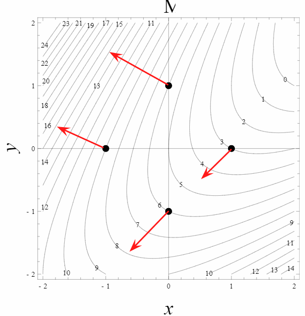
   Shown below is a contour plot of a scalar field, \(\mu(x,y)\). Assume that \(x\) and \(y\) are measured in meters and that \(\mu\) is measured in kilograms. Four points are indicated on the plot.
   

   

   1. Determine \(\frac{\partial\mu}{\partial x}\) and \(\frac{\partial\mu}{\partial y}\) at each of the four points.

      At each point, the partial derivative can be thought of as a ratio of the change in \(\mu\) when there is a small change in either \(x\) or \(y\) where the other variable is held constant (i.e., along either a horizontal or vertical line). To estimate a small change, we will use the smallest change available on the contour map: the change from the value at each indicated point to the nearest contour on both sides. This provides a slightly better estimate of the derivative than choosing only one side or the other, since the function may be changing more or less quickly in the positive or negative directions from the point. In cases where this is not possible due to the shapes of the contours, only the nearest side is used.
      

      Top: \begin{align} \frac{\partial \mu}{\partial x}&=\frac{\mu_+ - \mu_-}{x_+ - x_-} \approx\frac{5 - 7}{0.25 + 0.2}= -4.4 kg/m\\ \frac{\partial \mu}{\partial y}&=\frac{\mu_+ - \mu_-}{y_+ - y_-} \approx\frac{7 - 5}{1.4 - 0.2}= 0.8 kg/m \end{align}

      Left: \begin{align} \frac{\partial \mu}{\partial x}&=\frac{\mu_+ - \mu_-}{x_+ - x_-} \approx\frac{8 - 10}{-0.8 + 1.2}= -5 kg/m \\ \frac{\partial \mu}{\partial y}&=\frac{\mu_+ - \mu_-}{y_+ - y_-} \approx\frac{10 - 8}{0.4 + 1.1}= 1.3 kg/m \end{align}

      Bottom: \begin{align} \frac{\partial \mu}{\partial x}&=\frac{\mu_+ - \mu_-}{x_+ - x_-}=\frac{6 - 7}{0 + 0.6}= -1.7 kg/m \\ \frac{\partial \mu}{\partial y}&=\frac{\mu_+ - \mu_-}{y_+ - y_-}=\frac{5 - 7}{0 + 1.4}= -1.4 kg/m \end{align}

      Right: \begin{align} \frac{\partial \mu}{\partial x}&=\frac{\mu_+ - \mu_-}{x_+ - x_-} \approx\frac{3 - 4}{1 - 0.4}= -1.7 kg/m \\ \frac{\partial \mu}{\partial y}&=\frac{\mu_+ - \mu_-}{y_+ - y_-} \approx\frac{3 -4}{0 + 0.4}= -2.5 kg/m \end{align}

   2. On a printout of the figure, draw a qualitatively accurate vector at each point corresponding to the gradient of \(\mu(x,y)\) using your answers to part a above. How did you choose a scale for your vectors? Describe how the direction of the gradient vector is related to the contours on the plot and what property of the contour map is related to the magnitude of the gradient vector.

      Here is an example of what your graph could look like, pay particular attention to the fact that the gradient points uphill and is perpindicular to the contour lines (lines of contant mu). Also gradient vectors near larger densities of contour lines should be larger in magnitude since the contour lines being close correspond to steeper increases.

      

   3. Evaluate the gradient of \(h(x,y)=(x+1)^2\left(\frac{x}{2}-\frac{y}{3}\right)^3\) at the point \((x,y)=(3,-2)\).

      \begin{align} \vec{\nabla}h(x,y)\Bigg\vert_{(3,-2)} &= 2(x+1)\left(\frac{x}{2}-\frac{y}{3}\right)^3\, \hat{x} +3(x+1)^2\left(\frac{x}{2}-\frac{y}{3}\right)^2 \left(\frac{\hat{x}}{2}-\frac{\hat{y}}{3}\right)\Bigg\vert_{(3,-2)}\\ &=8\left(\frac{13}{6}\right)^3\, \hat{x} +48\left(\frac{13}{6}\right)^2 \left(\frac{\hat{x}}{2}-\frac{\hat{y}}{3}\right)\\ &=56 \left(\frac{13}{6}\right)^2\hat{x}-\frac{48}{3}\left(\frac{13}{6}\right)^2\hat{y}\approx 194 \hat{x}-75\hat{y} \end{align}