Problem-Solving: Fall-2024
W1 D3 Practice (SOLUTION): Due W1 D3
- Power Series Practice
S1 5139S
- Calculate the \(n=0, 1, 2, 3, 4\) coefficients of the power series for \(\cos{z}\) expanded around \(z=\pi\). Using these coefficients, find a power series approximation for this function.
First, the form of the answer will be: \[ \cos z \approx c_0 + c_1 (z-\pi) + c_2 (z-\pi)^2 + c_3(z-\pi)^3 + c_4(z-\pi)^4\]
Because I'm asked for the fourth order expansion, I'll keep only terms with power 4 or less.
Now, to calculate the coefficients: \begin{eqnarray*} c_0 &=& \frac{1}{0!}f(z=z_0) = \cos\pi = -1 \\ c_1 &=& \frac{1}{1!}\left.\frac{df}{dz}\right|_{z=z_0} = -\sin \pi = 0 \\ c_2 &=& \frac{1}{2!}\left.\frac{d^2f}{dz^2}\right|_{z=z_0} = -\frac{1}{2}\cos \pi = \frac{1}{2} \\ c_3 &=& \frac{1}{3!}\left.\frac{d^3f}{dz^3}\right|_{z=z_0} = \frac{1}{6}\sin \pi = 0 \\ c_4 &=& \frac{1}{4!}\left.\frac{d^4f}{dz^4}\right|_{z=z_0} = \frac{1}{24}\cos \pi = -\frac{1}{24} \\ \end{eqnarray*}
So, the approximation I end up with is:
\[ \cos z \approx -1 + \frac{1}{2} (z-\pi)^2 +-\frac{1}{24}(z-\pi)^4\]
- Plot both the original function and your approximation.
Here is the code in Mathematica and the graph it produces.
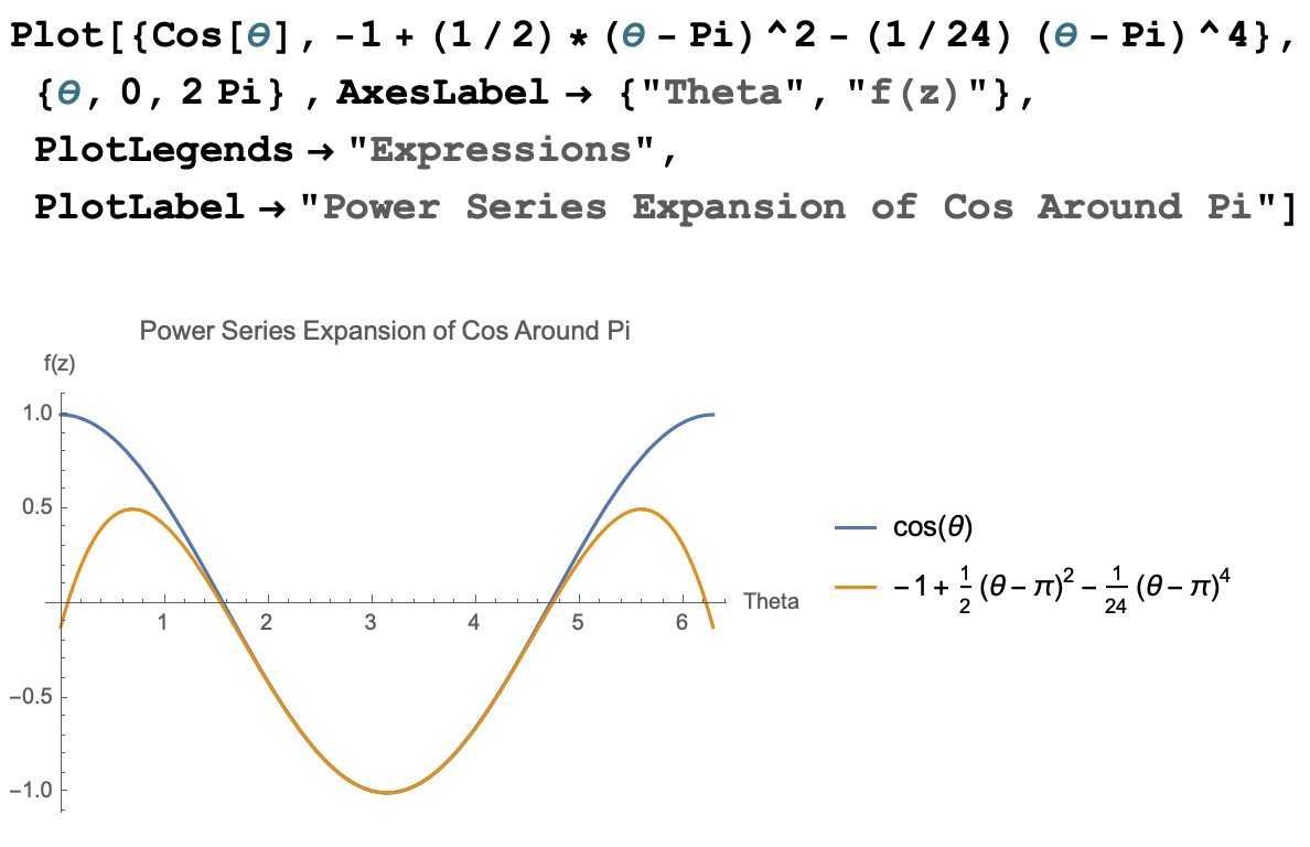
- For what values of \(z\) is your approximation “good”?
When I plot this approximation against the cosine function, I see that the expansion approximates the cosine function reasonably well between about \(\pi/2\) and \(3\pi/2\).
- Calculate the \(n=0, 1, 2, 3, 4\) coefficients of the power series for \(\cos{z}\) expanded around \(z=\pi\). Using these coefficients, find a power series approximation for this function.
- Sensemaking from Graphs of Power Series I
S1 5139S
- For the following graphs, identify the minimum order in a power series expansion that could accurately describe the curve for all values of the independent variable.
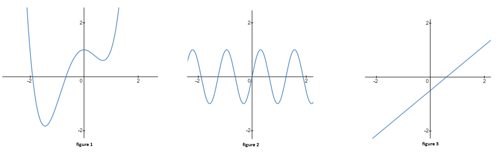
The leftmost graph has 3 turnaround points and must at minimum be of order 4. The middle graph is of \(\sin(x)\) and needs an infinite number of polynomial terms to accurately describe it for all values of \(x\). The far right graph is linear and only needs to go to order 1.
- For the following graphs, identify the minimum order in a power series expansion that could accurately describe the curve for all values of the independent variable.
- Approximating Functions with Taylor Series
S1 5139S
Go to The Geometry of Mathematical Methods' page on approximating power series and enter the following function into the GeoGebra applet in the figure at the bottom of the page. \begin{align} Function: \frac{7}{2}x - 3x^2 + x^3 - \frac{1}{9}x^4 +\frac{1}{180} x^5 - \frac{1}{1014} x^6 \end{align}
Answer the following questions about the above function using the applet, assuming the region where the function accurately represents a physical system is \(0 \leq x \leq 5\) (i.e. where both \(x\) and the function itself are positive).
- Set \(m=0\), then move \(a\) between \(0\) and \(5\) and describe in words what the \(m=0\) expansion order is telling you for each value of \(a\). Do the same for \(m=1\). Finally, do this for \(m=2\) and use what this series approximation does as a model to explain what will happen for expansions at all higher values of \(m\).
\(m=0\) gives the 1st term in the Taylor series, on the graph this is shown to be a horizontal line which gives the value of the function at the point \(x=a\) (the point we are expanding around). \(m=1\) gives the tangent line at \(x=a\) since it is the 1st order expansion (our Taylor series now looks like \(y=mx+b\), where \(b\) is the 1st term in the expansion and \(mx\) is the 2nd term). When we get to \(m=2\), we need to realize we're building something more complex, the "best fit" quadradic for the function at the point we are expanding around. For higher values of \(m\), we will have the “best fit” polynomial function for whatever order we have \(m\) equal to. For \(m=3\), we will make the “best fit” cubic around \(x=a\) and for \(m=4\) we will have the b"best fit" quartic around \(x=a\).
- Set the approximation to expand around \(x=0\). What is the minimum expansion order necessary to approximate the function within \(15\%\) of its actual value at \(x=2\)? What about within \(5\%\)? Verify these with a calculation.
For the \(15\%\) criterion, the minimum order appears to be \(m=4\), we can see this by plugging this into our 4th order expansion and our original function:
Original function at \(x=2\): \begin{align} \frac{7}{2}(2) - 3(2)^2 + (2)^3 - \frac{1}{9}(2)^4 +\frac{1}{180} (2)^5 - \frac{1}{1014} (2)^6=1.3369 \end{align} 4th Order Expansion at \(x=2\), this is just a truncated version of the original fucntion out to order 4: \begin{align} \frac{7}{2}(2) - 3(2)^2 + (2)^3 - \frac{1}{9}(2)^4 =1.222 \end{align} Now we take one minus the ratio to get the percent error: \begin{align} \% \;error=1-\frac{1.222}{1.3369}=0.086=8.6\% \end{align} This is under 15% so it works! For 5% we need to go out to m=5 and when we do we get: \begin{align} \frac{7}{2}(2) - 3(2)^2 + (2)^3 - \frac{1}{9}(2)^4 +\frac{1}{180} (2)^5 - \frac{1}{1014} (2)^6=1.3369\\ \frac{7}{2}(2) - 3(2)^2 + (2)^3 - \frac{1}{9}(2)^4 +\frac{1}{180} (2)^5=1.4 \end{align} Our standard error is then: \begin{align} \% \; error=\vert 1-\frac{1.4}{1.3369}\vert =\vert -0.047\vert=4.7\% \end{align} This just barely works! Also note we took the absolute value since percentage error can be in either direction. - Still expanding around \(x=0\), as you go from \(m=4\) to \(m=5\), does the term you're adding have a positive or negative coefficent? How do you know?
The term we added needs to be positive since the approximation is currently fitting below the original function. If we add a positive term, it will raise the approximate function up to more nearly meet the original one.
- Still expanding around \(x=0\), as you go from \(m=4\) to \(m=5\), is your approximation improving at \(x=2\)? What about \(x=4\)? Is this the behavior you expect? Explain.
For the point at \(x=2\) we seem to get a more accuate approximation. For \(x=4\), it actually becomes worse as we add the extra term. This happens because the Taylor Series approximation is attempting to better approximate points closer to \(x=0\), since that is the point we are expanding around, and points further from \(x=0\) are just following the trend from whatever power dominates the series (the highest ordered term will have the highest power) and so sometimes adding another term can lead to a better approximation further away but sometimes it does not, just like in this case.
- Set \(m=0\), then move \(a\) between \(0\) and \(5\) and describe in words what the \(m=0\) expansion order is telling you for each value of \(a\). Do the same for \(m=1\). Finally, do this for \(m=2\) and use what this series approximation does as a model to explain what will happen for expansions at all higher values of \(m\).