Problem-Solving: Fall-2024
Tutorial 1 (Required) (SOLUTION): Due W1 D4

1. Two Charges S1 5138S Sketch the equipotentials for two equal positive charges \(Q\) separated by a distance \(D\). Make sure to state the reasons for the main features of your sketch. You may use technology to check your answer, but you still need to state reasons for the features. Note: It is an important convention that the VALUES of contour lines should be equally spaced.
2. Potential vs. Potential Energy S1 5138S

   In this course, two of the primary examples we will be using are the potential due to gravity and the potential due to an electric charge. Both of these forces vary like \(\frac{1}{r}\), so they will have many, many similarities. Most of the calculations we do for the one case will be true for the other. But there are some extremely important differences:

   1. Find the value of the electrostatic potential energy of a system consisting of a hydrogen nucleus and an electron separated by the Bohr radius. Find the value of the gravitational potential energy of these two particles at the Bohr radius. Use the same system of units in both cases. Compare and the contrast the two answers.

      Bohr radius: \(a_0\approx 0.0529~\textrm{nm}\)
      Proton charge: \(Q\approx 1.60\times 10^{-19}~\textrm{C}\)
      

      \begin{equation*} \frac{1}{4\pi\epsilon_0}\approx 9.0\times 10^{9}~\textrm{Nm}^2/\textrm{C}^2 \end{equation*}

      Gravitational constant: \(G\approx 6.67\times 10^{-11}~\textrm{Nm}^2/\textrm{kg}^2\)
      Proton mass: \(M\approx 1.67\times 10^{-27}~\textrm{kg}\) Electron charge: \(q\approx -1.60\times 10^{-19}~\textrm{C}\)
      Electron mass: \(m\approx 9.11\times 10^{-31}~\textrm{kg}\)
      Therefore:

      \begin{align*} U_{\textrm elec} &= qV_{\textrm elec}\\ &= \frac{1}{4\pi\epsilon_0}\frac{qQ}{a_0}\\ &\approx -4.35\times 10^{-18}~J \\ U_{\textrm grav} &= mV_{\textrm grav}\\ &= -G \frac{mM}{a_0}\\ &\approx -1.92\times 10^{-57}~J \end{align*}

      The potential energy due to gravity in an atom is 28 orders of magnitude smaller than the electromagnetic force! (Notice that \(qV_{\textrm elec}\) is not the binding energy of the electron. The electron in the Bohr model also has kinetic energy.)

   2. Find the value of the electrostatic potential due to the nucleus of a hydrogen atom at the Bohr radius. Find the gravitational potential due to the nucleus at the same radius. Use the same system of units in both cases. Compare and contrast the two answers.

      See constants above. Therefore:

      \begin{align*} V_{\textrm elec} &= \frac{1}{4\pi\epsilon_0}\frac{Q}{a_0}\approx 27.2~\textrm{J}/\textrm{C}\\ V_{\textrm grav} &= -G \frac{M}{a_0} \approx -2.11\times 10^{-27}~\textrm{J}/\textrm{kg} \end{align*}

      Even though these are measured in the same system of units, they are not in the same units and cannot be compared.

   3. Briefly discuss at least one other fundamental difference between electromagnetic and gravitational systems. Hint: Why are we bound to the earth gravitationally, but not electromagnetically?

      One difference is that charges of both signs exist, so that electromagnetic forces can cancel each other. The earth is essentially electromagnetically neutral, so that we do not feel an electromagnetic attraction to the earth. (Be careful, the earth is essentially electromagnetically neutral ON AVERAGE. However, there can be largish charge differences locally--this is what causes lightening, for example.) Gravitational forces, however, can only add, so that the total force due to lots of mass can be very large.

      Another difference is that masses always attract, so that the gravitational potential is negative. Whereas, positive charges repel each other so that the electrostatic potential of a positive charge is positive.

3. Series Convergence S1 5138S

   Recall that, if you take an infinite number of terms, the power series for \(\sin z\) and the function itself \(f(z)=\sin z\) are equivalent representations of the same thing for all real numbers \(z\), (in fact, for all complex numbers \(z\)). This is what it means for the power series to “converge” for all \(z\).
   

   Not all power series converge for all values of the argument of the function. More commonly, a power series is only a valid, equivalent representation of a function for some more restricted values of \(z\), even if you keep an infinite number of terms. The technical name for this idea is convergence--the series only "converges" to the value of the function on some restricted domain, called the “interval” or “region of convergence.”

   1. Find the power series for the function \(f(z)=\frac{1}{1+z^2}\) expanded around \(z=0\)..

   2. Using the Geogebra applet from class as a model, or some other computer algebra system like Mathematica or Maple, plot both the original function and the power series to explore the convergence of this series. Where does your series for this new function converge? Can you tell anything about the region of convergence from the graphs of the various approximations?
      

      Print your plot and write a brief description (a sentence or two) of the region of convergence.
      

      You may need to include a lot of terms to see the effect of the region of convergence. You may also need to play with the values of \(z\) that you plot. Keep adding terms until you see a really strong effect!

   Note: As a matter of professional ettiquette (or in some cases, as a legal copyright requirement), if you use or modify a computer program written by someone else, you should always acknowledge that fact briefly in whatever you write up. Say something like: “This calculation was based on a (name of software package) program titled (title) originally written by (author) copyright (copyright date).”

   Investigating the series for \(f(z)=\frac{1}{1+z^2}\), I can see it is of the form of \((1+z)^p\), this is one of our (hopefully) memorized common power series, to get it fully in that form, I'll change the way it looks:

   \[f(z)=\frac{1}{1+z^2}=(1+z^2)^{-1} \]

   Now I can see \(p=-1\) and our power series \(z\)'s role is filled by \(z^2\) in this function. So I can apply the power series formula for\(f(z)=\frac{1}{1+z^2}\) to get:

   \[f(z)=\frac{1}{1+z^2}=1-z^2+z^4-z^6...\]

   I can see the pattern (all coefficients either 1 or -1 with alternating signs) from this many terms. Now I'll investigate the graph:

   

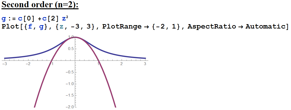
   I see the original function in blue, and the power series approximation to order 2 in purple. I can see the power series approximates the original function reasonably well for \( -0.5<z<0.5\). Typically when you add more terms to a power series approximation, it will become a better approximation further away from its center point with each added term, but only until you reach the edge of the region of convergence. I'll look at what happens went I include 50 terms (with the help of technology!!):

   

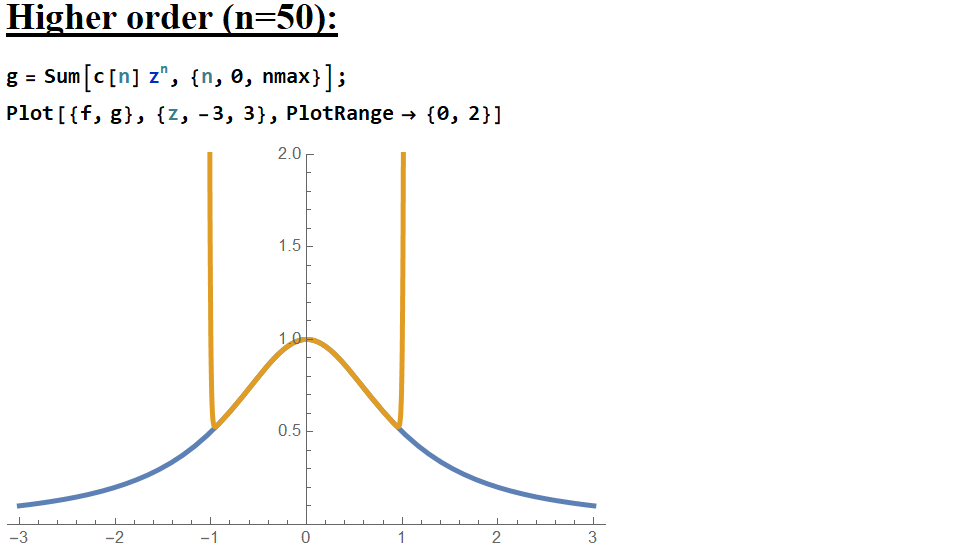
   Now I see that the power series is a better approximation to the function, but only out to \(\vert z\vert=1\), and afterwards the actual behavior in fact curves AWAY from the original function MORE with each additional term! A surprising result! When I learned the series for \((1+z)^p\), I was given the condition that \(|z|\leq1\), and here I can see that playing out! Not only does the power series only converge when \(|z|\) is less than 1, it actively diverges afterward, more aggressively with every added term!